ODI in the hybrid database world – Amazon Redshift – AWS CLI

Posted in AWS, Cloud, ODI with tags , , on June 5, 2023 by Rodrigo Radtke de Souza

Written on June 5, 2023 by Rodrigo Radtke de Souza

Hi all, probably this is the last post of this series on how to load data from on-premises databases to the major public clouds providers. Today’s post is about Amazon Redshift. Right now, we all know the pattern that we are following: We will duplicate “IKM SQL to File Append” and add some extra steps at the end of it to push the file to the cloud and load the target table. It will look like below:

The first extra command is GZIP, which is the same as the other posts. After we GZIP the file, we will push the file to a S3 bucket using the CP command. To do that, you will need to create a S3 bucket in AWS and install AWS CLI (which you can read about it here) in your ODI server. The AWS CP command is very simple and looks like this:

The next command (aws redshift-data) is a little more complex. redshift-data is an API (read about it here) used to manipulate data in redshift. One of its commands is execute-statement (read about it here), which can be used to issue a copy command (read about it here), that copies a file from a S3 bucket to a redshift table.

The command may vary depending on your setup, but in resume, it will look like this:

aws redshift-data execute-statement --database <database_name> --workgroup-name <workgroup_name> --region <region> --secret-arn <secret_arn> --sql "copy <target_table> from 's3://<bucket>/<file_name>.gz' credentials 'aws_access_key_id=<access_key_id>;aws_secret_access_key=<access_key_secret>' delimiter '|' IGNOREHEADER 1 ACCEPTINVCHARS GZIP region '<region>'"

Notice that there are a lot of variables to fill in. secret_arn, access_key_id and access_key_secret are all related to security and depending on your setup, you may even use different ways to authenticate and run the command. But in resume, you will request redshift-data api to run a execute-statement. This execute-statement will trigger a copy command to a target table from a s3 bucket GZIP file. When you run the mapping, it looks like this:

That’s it folks. I hope you have enjoyed this series. See you next time!

ODI in the hybrid database world – Azure SQL Database – BCP Utility

Posted in Cloud, ODI with tags , , on May 8, 2023 by Rodrigo Radtke de Souza

Written on May 8, 2023 by Rodrigo Radtke de Souza

Hi all! Continuing the ODI in the hybrid database world series, let’s talk today about Azure SQL Database. This one is the simplest so far in our series, but it has some limitations.

The process is again like what we have been doing for some time now. We will duplicate “IKM SQL to File Append” and add some extra steps at the end of it to push the file to the cloud and load the target table. In the Azure SQL Database case, we will only need the BCP Utility installed in the ODI agent server. You can read about BCP Utility here.

The limitation of using this utility (at least I didn’t find anything different than that) is that it does not work with a compressed file, which ends up sending the entire file over the internet in batch sizes (which is configurable). I found a solution that you could first load a compressed file to an Azure Blob storage and then use Azure Data Factory to load this compressed file to Azure SQL Database, but this kind of breaks the simplicity of the examples that we are presenting here in this series, so I won’t go over that example. This is how the IKM will look like:

The first five steps are from the original SQL to File Append IKM. The only new is the one that calls BCP.  This step is very straightforward:

You need to pass the table name in Azure SQL that you want to load, the path to the text file that you created in ODI, the SQL Server name (which will look like this: <MY_SQL_SERVER>.database.windows.net), the database name and finally the Azure SQL user and password that you want to use to connect to the cloud database. There are some additional parameters that indicates some information about the file, like -t “|” that indicates that this is a pipe delimited file and -F 2, which indicates that the data rows begin in the second line of the file, since the first one is the header.

When you run the mapping, you see the following:

If you open the logs, you are going to see that it sent the data in 1000 batches:

The batch size and some more interesting parameters can be seen in the BCP documentation. You may play around with them and see which one is better for your specific data load.

See you next time!

ODI in the hybrid database world – Oracle ADW – OCI/CLI + DBMS_CLOUD

Posted in Autonomous Database, Cloud, ODI with tags , , on April 14, 2023 by Rodrigo Radtke de Souza

Written on April 14, 2023 by Rodrigo Radtke de Souza

Hi! In all the previous posts about ODI in the hybrid database world, I always showed two versions of data loads for each technology, one being JDBC and another with text files. In the case of Oracle ADW, I posted just the JDBC example. So, let me correct that today. Let’s see how you can also use text files to load data into Oracle ADW tables.

The process is very similar to what we have been doing for some time now. We will duplicate “IKM SQL to File Append” and add some extra steps in the end of it to push the file to the cloud and load the target table. In the ADW case, we will need a couple of things to make it work:

  • An Oracle Bucket, which is a container for storing objects in a compartment within an Object Storage namespace in the Oracle cloud. More information about it here.
  • Install OCI CLI, which ODI will call to push the file to the Oracle Bucket. The steps on how to install it can be found here.

Those two you will need to create and install before proceeding. There is a third component needed, but this one already exists in the Oracle ADW: DBMS_CLOUD package. You may read about it here.

This package will be used to push the data from Oracle Bucket to Oracle ADW table. There is a configuration that you may need to do regarding DBMS_CLOUD credentials, but I’ll talk about it later.

This is what the final IKM will look like:

First five steps are from the original KM. The last three are brand new. Let’s take a look first on GZIP:

Here we are just zipping the text file before sending it to the cloud. Just notice that Oracle accepts other kinds of compression, so you may change it if you want to. I used GZIP because it seems to be a standard that works with all Public cloud vendors out there.

Next one is OCI PUT:

Very straight forward step that gets the GZIP file and uses OCI CLI to PUT the file in an Oracle Bucket that belongs to an Oracle NameSpace. You may refer to OCI PUT documentation here.

Last one is dbms_cloud copy_data step:

COPY_DATA may have other options. A full list can be found here.

All options are self explanatory. In this case we are loading a text file with columns separated by pipes (“|”). One option that you need to notice is file_uri_list. It indicates the text file URL that resides in your Oracle bucket. It may look like this:

https://swiftobjectstorage.region.oraclecloud.com/v1/namespace-string/bucket/filename

or like this:

https://objectstorage.region.oraclecloud.com/n/namespace-string/b/bucket/o/filename

To make things simpler in this example, I set the bucket as public, so I could access it without credentials. However, in a production environment, that won’t be the case and you will need to create a credential using DBMS_CLOUD.create_credential. You will run this command only once in your Oracle ADW instance:

begin
  DBMS_CLOUD.create_credential (
	credential_name => 'OBJ_STORE_CRED',
	username => 'XXXXX',
	password => 'YYYYY'
  ) ;
end;

You can read more about how to create the credential here. After you create the credential, you will use it in the COPY_DATA command as a parameter (credential_name).

When we run the mapping, we get something like this:

Very similar to the other posts, we are generating a text file, GZIPing it, calling OCI CLI to send the file to the cloud and then calling DBMS_CLOOUD.COPY_DATA procedure to load the data from the Oracle bucket to our target table.

I hope you liked it! See you next time!

Snowflake loader using ODI

Posted in ODI, Snowflake with tags , on April 13, 2023 by Rodrigo Radtke de Souza

Written on April 13, 2023 by Rodrigo Radtke de Souza

Hi all. Today’s post will talk about how to create a simple, but powerful Snowflake loader using ODI. Actually, you may use it with any technology that you want, but I ended up creating this one for Snowflake because I needed to load several Oracle tables to Snowflake in a fast and dynamic manner.

This post combines the techniques described here and here. In the first post we saw how to load text files to Snowflake. In the second post we saw how to create dynamic text dumps from Oracle. What if we combine both posts? We could create a dynamic load that will receive a table name as a parameter, create a text file and push this text file to Snowflake. Isn’t that cool?

Our dynamic loader will be an ODI Procedure and it will have the following steps:

You can get the code for “Get File Metadata”, “Create File”, “Truncate File”, “Create Header” and “Insert Rows” from my past post. There is a new step here called “Create target table” that will try to create a table in Snowflake if it does not exists yet. I added this step just as a convenient way to speed up my development process, since this procedure is nothing more than a job to get some table from Oracle and copy that to Snowflake. The code is below:

CREATE TABLE <%=odiRef.getSchemaName( "D" )%>.<@=table_name@>
(
<@=table_column_type@>
);

Just don’t forget to set the target schema with the logical schema from Snowflake where you want the table to be created and also set “Ignore Errors” in the procedure, so if the table exists it does not stop the process.

The last three steps are almost the same as in the first post, with one change. Instead of <%=odiRef.getTargetTable(“TABLE_NAME”)%>, now I’m getting the information from <@=folder_path@> and <@=table_name@>. E.g:

OdiOSCommand "-OUT_FILE=<@=folder_path@>_copy.log" "-ERR_FILE=<@=folder_path@>_copy.err"
snowsql -c #P_CONNECTION_NAME -w #P_SNOW_WAREHOUSE -r #P_SNOW_ROLE -d #P_SNOW_DATABASE -s #P_SNOW_SCHEMA -q "copy into #P_SNOW_DATABASE.#P_SNOW_SCHEMA.<@=table_name@> from  @#P_STAGE_NAME/<@=table_name@>.gz"

When we execute the package, we have the following:

The job received a table name as a parameter. It gets the metadata from the table name in Oracle, creates a file with its data, gzips it, sends it to Snowflake using PUT and COPY it into the final table (that was created for you if it didn’t exist before). Awesome right? If you notice it, this process will duplicate the data if you run it twice, since it does not truncate the target table before loading the data into it. I did that on propose because there was scenarios that I wanted to load several different datasets into a single table, in append mode. But, you may enhance this procedure and add a step to truncate the target table if you wish.

Hope you enjoyed! See you next time!

Building dynamic ODI code using Java variables – Table to File example

Posted in ODI with tags , on March 23, 2023 by Rodrigo Radtke de Souza

Written on March 23, 2023 by Rodrigo Radtke de Souza

Hi all. Today’s post is an “enhancement” of one post that I did a long time ago regarding using Oracle’s metadata to build dynamic code. I say it is an enhancement because that technique would use the source/target command tabs and it has a 4000 character limitation. So, if you are trying to build some metadata information that crosses this limit, it will fail.

You should be good using source/target command technique in 90% of your data loads, but there are a few exceptions that we need to go beyond 4000 characters. One of these examples is when you are trying to build dynamic code to generate text file loads in ODI. The example that I’ll show here is about dumping the data from any Oracle table to a text file dynamically, using only one ODI procedure.

This is what we will build. I’ll go over each step in detail:

Basically, it is an ODI procedure that will receive a table name as a parameter and it will write that table data into a text file using pipe “|” as delimiters. This is a very small but useful procedure that you may use when you need to create fast text files from tables/views without going through all the work to create ODI mappings for it.You will need two Logical Schemas, one for the source table and another one for the target file. In this example I used LOCAL_SOURCE that points to an Oracle database and OUTPUT_FILE that points to a folder where the text file will be created.First step is to get the file metadata. As I said, this will be done in a different way now. Instead of using source/target tab commands, we will use Java BeanShell to retrieve this information. This is because ODI creates a very lengthy metadata for each column and the total amount of metadata often crosses the 4000 characters limit. Just as an example, each column in a file text load looks similar to this:

"CRDWG_COLSNP$CRCOL_NAME="+metaDataSrc.getColumnName(i) + "SNP$CRTYPE_NAME=STRINGSNP$CRORDER="+i+"SNP$CRLENGTH=4000SNP$CRPRECISION=4000SNP$CRACTION_ON_ERROR=NULLSNP$"

Here is the full code for the “Get File Metadata” step:

<@
import java.sql.*;

String table_name = "#DWCLOUD.L_TABLE_NAME";
String folder_path = odiRef.getSchemaName("OUTPUT_FILE","D")+"/"+table_name;
String folder_path_txt = folder_path+".txt";
String table_schema = odiRef.getSchemaName("LOCAL_SOURCE","D");
String table_metadata = "/*$$SNPS_START_KEYSNP$CRDWG_TABLESNP$CRTABLE_NAME="+table_name+"SNP$CRLOAD_FILE="+folder_path_txt+"SNP$CRFILE_FORMAT=DSNP$CRFILE_SEP_FIELD=0x007cSNP$CRFILE_SEP_LINE=0x000D0x000ASNP$CRFILE_FIRST_ROW=1SNP$CRFILE_ENC_FIELD=SNP$CRFILE_DEC_SEP=SNP$CRSNP$";
String table_header = "";
String table_header_parameter = "";

Connection ConSrc = DriverManager.getConnection("<%=odiRef.getInfo("SRC_JAVA_URL")%>","<%=odiRef.getInfo("SRC_USER_NAME")%>",odiRef.getInfo("SRC_PASS"));
Statement stmtSrc = ConSrc.createStatement();
ResultSet querySrc =  stmtSrc.executeQuery("select /*+ parallel(64) */ * from "+ table_schema +"." + table_name + " where 1=2");
ResultSetMetaData metaDataSrc = querySrc.getMetaData();

int count = metaDataSrc.getColumnCount();
for (int i=1; i<=count; i++)
  {
	table_metadata = table_metadata + "CRDWG_COLSNP$CRCOL_NAME="+metaDataSrc.getColumnName(i) + "SNP$CRTYPE_NAME=STRINGSNP$CRORDER="+i+"SNP$CRLENGTH=4000SNP$CRPRECISION=4000SNP$CRACTION_ON_ERROR=NULLSNP$";
	table_header = table_header+metaDataSrc.getColumnName(i);
	table_header_parameter = table_header_parameter+":"+metaDataSrc.getColumnName(i);  
    	 
	if (i==count)
	{
  	table_metadata=table_metadata+"CR$$SNPS_END_KEY*/";
	} else
	{   
  	table_metadata=table_metadata+"CRSNP$";
  	table_header = table_header + ",";
  	table_header_parameter = table_header_parameter + ",";    
	}
  }

ConSrc.close();
@>

How it works? It uses a variable (that you will use in an ODI package later on), to figure out which table it will dump into a file. It actually can be other objects that you can query, like a view. Views are actually great to be used here since you may create any kind of business logic and filters on the view and dump the data to a file when needed. It also uses both logical schemas (source and target) to figure out where to read the source data and place the target file.

It then creates a connection object using the source connection that you set in the ODI procedure (please pay close attention to each source/target logical schema in the ODI procedure) and it runs a query where 1=2 just to retrieve the table/view metadata.

Having this metadata in the result set, it loops through it and starts to “build” the dynamic code for the header and the columns. It does some special conditions when it reaches the last column and then it closes the connection.

It may sound complicated, but it’s fairly simple. In less than 40 lines of code we are able to retrieve all metadata to dump any table’s data to a flat file in a dynamic way. The other steps are now very straight forward.

“Create File” step will be as simple as this:

create table "<@=folder_path@>"
<@=table_metadata@>

Same for “Truncate File”:

truncate table "<@=folder_path@>"
<@=table_metadata@>

“Create Header”:

create header (<@=table_header@>)
<@=table_metadata@>

“Insert Rows” is the only one that needs two steps. In Source Command we have:

select     
    /*+ parallel(64) */ <@=table_header@>
from    <@=table_schema@>.<@=table_name@>
where    
    (1=1)    

This one is used to read the source table. In Target Command we have the insert statement to the file object:

insert into "<@=folder_path@>"
(
	<@=table_header@>
)
values 
(
	<@=table_header_parameter@>
)
<@=table_metadata@>
  

Add this procedure in an ODI package, alongside with the ODI variable for the table name:

Add the table/view object that you want to dump the records. In this example, I used a table named SAMPLE_DATA. When I executed the package, I have the following:

If I go to the folder path defined in OUTPUT_FILE logical schema, I can see the data file created there (they are all fake/random rows, not real people information):

I hope you liked this post. See you soon!

ODI Hidden Gems – SNP tables: Query to get load plan execution steps

Posted in ODI, Query with tags , on December 6, 2022 by Rodrigo Radtke de Souza

Hi all,

Today is a short post, but very useful. I often get asked about how to write SNP table queries to get some information from ODI repositories. I posted one about “executed code” here. Today, this is another example of how to get a load plan execution steps that were executed. This one I use in the end of every load plan execution, so it creates a mini report of how each step performed in that load plan. This is useful for ODI Operators, so they can do some analysis of how well their jobs are doing.

This query was created using ODI 12.2.1.4.

WITH 
LP_STEPS AS (
SELECT SLS.I_LOAD_PLAN
     , LP.LOAD_PLAN_NAME
     , I.I_LP_INST
     , SLS.LP_STEP_NAME
     , SLS.I_LP_STEP
     , SLS.PAR_I_LP_STEP
     , SLS.STEP_ORDER
     , LEVEL AS LEVEL_
     , SYS_CONNECT_BY_PATH(SLS.LP_STEP_NAME, ' -> ') AS STEP_NAME_PATH
     , SYS_CONNECT_BY_PATH(SLS.STEP_ORDER, ' ') AS STEP_ORDER_PATH
     , SYS_CONNECT_BY_PATH(SLS.IND_ENABLED, ' ') AS IND_ENABLED_PATH
     , SYS_CONNECT_BY_PATH(DECODE(SLS.LP_STEP_TYPE, 'EX', 1, 0), ' ') AS EXCEPTION_STEP_PATH
     , CONNECT_BY_ISLEAF IS_LEAF
     , SLS.IND_ENABLED
  FROM SNP_LOAD_PLAN LP
    INNER JOIN SNP_LP_STEP SLS
        ON SLS.I_LOAD_PLAN = LP.I_LOAD_PLAN
    INNER JOIN SNP_LP_INST I
        ON SLS.I_LOAD_PLAN = I.I_LOAD_PLAN
        AND I.GLOBAL_ID = '<LOAD_PLAN_INSTANCE_GLOBAL_ID_HERE>'
 CONNECT BY PRIOR SLS.I_LP_STEP = SLS.PAR_I_LP_STEP 
  START WITH SLS.PAR_I_LP_STEP IS NULL
)  
, ALL_ AS (
SELECT L.I_LOAD_PLAN
     , L.LOAD_PLAN_NAME
     , L.I_LP_INST
     , L.LP_STEP_NAME
     , L.I_LP_STEP
     , L.STEP_NAME_PATH
     , L.STEP_ORDER_PATH
     , CASE WHEN L.IND_ENABLED_PATH LIKE '%0%' THEN 'N' ELSE 'Y' END ENABLED
     , MAX(IL.SESS_NO) AS SESS_NO
  FROM LP_STEPS L
    LEFT JOIN SNP_LPI_STEP_LOG IL
        ON L.I_LP_INST = IL.I_LP_INST
        AND L.I_LP_STEP = IL.I_LP_STEP
 WHERE 1 = 1
   AND L.IS_LEAF  = 1
   AND EXCEPTION_STEP_PATH NOT LIKE '%1%'
 GROUP BY L.I_LOAD_PLAN
        , L.LOAD_PLAN_NAME
        , L.I_LP_INST
        , L.LP_STEP_NAME
        , L.I_LP_STEP
        , L.STEP_NAME_PATH
        , L.STEP_ORDER_PATH 
        , L.IND_ENABLED_PATH
) 
SELECT A.I_LOAD_PLAN
     , A.I_LP_STEP
     , A.LOAD_PLAN_NAME
     , A.LP_STEP_NAME
     , A.STEP_NAME_PATH
     , A.SESS_NO
     , CASE WHEN A.ENABLED = 'N' THEN 'Step has been disabled'
            WHEN A.SESS_NO IS NULL THEN 'Step did not run'
            WHEN S.SESS_STATUS = 'D' THEN 'Step finished successfully'
            WHEN S.SESS_STATUS = 'E' THEN 'Step failed'
            WHEN S.SESS_STATUS = 'W' THEN 'Step finished with warnings'
            ELSE 'Other status not relevant'
        END STATUS
     , TO_CHAR(S.SESS_BEG, 'DD-MON-YYYY HH24:MI:SS') AS SESS_BEG
     , TO_CHAR(S.SESS_END, 'DD-MON-YYYY HH24:MI:SS') AS SESS_END
     , S.SESS_DUR
     , REPLACE(REPLACE(REPLACE(SUBSTR(S.ERROR_MESSAGE, 1, INSTR(S.ERROR_MESSAGE, CHR(9) || 'at ')), CHR(10), ' '), CHR(13), ' '), CHR(9), ' ') AS ERROR_MESSAGE
  FROM ALL_ A
    LEFT JOIN SNP_SESSION S
        ON A.SESS_NO = S.SESS_NO
 ORDER BY A.STEP_ORDER_PATH;

I hope you like it! See you soon!

ODI in the hybrid database world – Google BigQuery – gsutil + bq

Posted in BigQuery, Cloud, Google, ODI with tags , , on December 5, 2022 by Rodrigo Radtke de Souza

As we saw in our last post, ODI + BigQuery + Simba Jdbc didn’t give us the performance that we were expecting. But we may apply the same concept that we did for Snowflake: we may create a file, zip it (using GZIP), send it to a storage location (using gsutil) and load it into a table (using bq). Luckily, this is easy to do in ODI and Bigquery. First, we will need to install Google Cloud CLI, which will enable you to use both gsutil and bq. You may read about it here.

Next, we will follow the same steps that we did for Snowflake, first we will create a copy of an existing IKM. In this case, I duplicated IKM SQL to File Append and gave it a new name:

On Tasks, I left some original ones (which will create a text file for us) and I created three new steps: GZIP, Copy and Load.

The first new step is GZIP, because we want to compress our file before moving it to the cloud. Google BigQuery may load zipped files directly from Cloud Storage, but they need to be in a GZIP format. So, on “Target Command” I added this:

OdiOSCommand "-OUT_FILE=<%=odiRef.getTable("TARG_NAME")%>_zip.log" "-ERR_FILE=<%=odiRef.getTable("TARG_NAME")%>_zip.err"

"C:\Program Files\7-Zip\7z.exe" a "<%=odiRef.getTable("TARG_NAME")%>.GZ" "<%=odiRef.getTable("TARG_NAME")%>.txt"

For the sake of simplicity in this example, the path is hardcoded, but in a real-world project, we would make this path dynamic.

Second one is GCS Copy. In this step, we will call “gsutil cp” command that will get a file (in this case GZIP file that we created in the previous step) and send it to a bucket in Google Cloud Storage:

OdiOSCommand "-OUT_FILE=<%=odiRef.getTable("TARG_NAME")%>_cp.log" "-ERR_FILE=<%=odiRef.getTable("TARG_NAME")%>_cp.err"
gsutil cp "<%=odiRef.getTable("TARG_NAME")%>.GZ" gs://<YOUR_GCS_BUCKET_NAME_HERE>

Last step is using “bq load” command that will get the file that is stored in your bucket and load it to a table in BigQuery:

OdiOSCommand "-OUT_FILE=<%=odiRef.getTable("TARG_NAME")%>_bq.log" "-ERR_FILE=<%=odiRef.getTable("TARG_NAME")%>_bq.err"
echo bq load --source_format=CSV --skip_leading_rows=1 --field_delimiter="|" GOOGLE_TARGET.SAMPLE_DATA gs:// <YOUR_GCS_BUCKET_NAME_HERE>/SAMPLE_DATA.GZ| C:\WINDOWS\system32\cmd.exe /k ""C:\Users\<YOUR_USER>\AppData\Local\Google\Cloud SDK\cloud_env.bat""

This command is a little messy, but it works. In your project you may do something more elaborate, but for the sake of this example, it will work. Basically, I’m using the echo trick to call two command lines at once. The first one I run “cloud_env.bat”, which will set my cloud environment variables (this comes with Google CLI installation). Then, I call “bq load”, passing as parameters the source format, the number of heading lines and the field delimiter. In this case, we are using pipe “|” as our column delimiter. After that we pass which Dataset/Table we want to load and from which file (in this case our GZ file).

Seems complicated at first, but the data load speed is worth it. And since all this is in an IKM, you will do it once and reuse it repeatedly.

Before we create a mapping, we need to remember that now we won’t be loading BigQuery directly, but instead we will be loading a text file first. So, we need to create a new model pointing to a File logical schema that will be used to hold our temporary files. For this example, I’ve created a delimited file using pipe and with header. For the columns, I created all of them as Strings.

Now we may create our mapping. In this case, its pretty simple. We just add our Oracle source table and our File target table.

When we execute it, we can see that I was able to load 1,077,500 rows in 76 seconds. Not bad at all:

Once again, we saw that working with files and command line tools were way faster than JDBC connections. Also, if you think a little bit about it, it has other cool benefits. If you threat all your cloud integrations as file transfers, you may create an architecture that can be used across multiple cloud vendors. Your on-premises output will always be compressed files that will be loaded to cloud systems using different ODI Knowledge modules, one for each vendor. Since all of it are text files, ODI mappings may be used to create all sorts of complex logic using your on-premises database as staging and then only pushing the result to the cloud.

I hope you have enjoyed. See you soon!

ODI in the hybrid database world – Google BigQuery – Simba JDBC

Posted in BigQuery, Cloud, ODI with tags , on November 23, 2022 by Rodrigo Radtke de Souza

Hi all! Continuing our series, today we will talk about how to load data into BigQuery using ODI. There will be two posts, one talking about Simba JDBC and another one talking about Google Cloud SDK Shell. You will notice that the first approach (using Simba JDBC) has a lot of challenges, but I think its worth looking at it, so you have options (or at least know why you should avoid it).

First, you need to download Simba JDBC and add it to your ODI client/agent (like what was done with Snowflake JDBC here). Also, you need to “duplicate” one ODI technology (I used Oracle in this example) and name it as BigQuery:

In JDBC Driver, you will add the Simba driver and in URL you will add your connection to Google BigQuery. I’ll not go over the details here, since there are a lot of ways for you to create this URL, but you may check all the ways to create it in this link.

Press “Test Connection” to see if it is all working as expected:

Create a new Physical schema and give it the name of your BigQuery Dataset:

Create a new Logical Schema and a Model. If all is correct, you will be able to Reverse Engineer as you normally do with other technologies:

Let’s go ahead and just create a new mapping. This is a simple one: getting data from an Oracle database and loading it to BigQuery:

As LKM, I’m using LKM SQL to SQL:

As IKM, I just used a Global one:

When I ran it, it fails. If we check Operator, we will see that it couldn’t insert new rows because it was not able to create the C$ temporary table. If we look further, we see that it considers “$” as an illegal character in BigQuery tables:

If we get the create table statement from ODI Operator and try to execute in BigQuery, we will see a lot of issues with that:

First, as I said before, we cannot have $ signs, so let’s try to remove it:

It also does not accept NULL. Removing them gave another error:

Varchar2 is not a thing in BigQuery, so if we change it to String, it will work fine:

So, just for us to create a temporary C$ tables, we had to do several changes to it. It means that ODI/BigQuery integration is not straightforward as we did for Oracle Cloud or Snowflake. We will have to do some changes and additions to BigQuery technology in ODI. Let’s start with $ signs. Double click BigQuery and go to Advanced tab. There, lets remove the $ sign from temporary tables (I removed only in C$ for this example):

Also, you need to remove the DDL Null Keyword:

You may need to do way more changes depending on what you need to load, but for this example, we will try to keep as simple as possible.

Next step is to create a String Datatype. You may go to BigQuery technology and duplicate and existing Datatype. For this example, I used Varchar2. Then I changed the Name/Code/Reverse Code/Create table syntax/Writable Datatype syntax.

Another step is to change our source technology, in this case Oracle. We need to do that because ODI needs to know what to do when converting one datatype from one technology to another. We do this by going to Oracle Technology and double clicking in each source datatype that we have and what they compare to the new target technology (BigData). For this example, we will only be getting Varchar2 columns to String columns, so we will just make one change. In a real-world scenario, you would need to change all the ones that you use. Double click Oracle’s VARCHAR2 Datatype, click on “Converted To” tab and select String on BigQuery Technology.

One last change is to go to our BigQuery datastore and change the column types to String:

This should be enough for us to test the interface again. When we run it, no error happens this time:

However, the data load takes forever to complete (I cancelled after some hours trying to run a 1 M rows table). The ODI job was able to create the work table and I could see data flowing in BigQuery, but the speed was just too slow:

I tried to change the Array Fetch/Batch Update size/Parallelism in the Google BigQuery Data Server ODI object, but none of the values that I tried seemed to work fast as I wish:

Not sure if the slowness was due to something in my architecture, but at this point I just thought that, even if worked reasonably fast, it wouldn’t be as fast as creating a file and send it directly to BigQuery (similarly on what we did for Snowflake). Also, the amount of customization is so high to load a simple table, that I really don’t want to think on how bad it will get when we get to some complex mappings.

Not surprisingly, my tests with text files were extremely fast and the customizations needed are minimum compared to the JDBC method, so that’s what we will be covering in the next post.

Thanks! See you soon!

ODI in the hybrid database world – Files/Stages and SnowSQL

Posted in Uncategorized on April 14, 2022 by Rodrigo Radtke de Souza

Hi all, as mentioned in the second post of this series, there is a faster way to load data into Snowflake using ODI. It will require the creation of new KM, it has some peculiarities that some may think as limitations at first but the speed of the data loading is totally worth the work and the preparations needed for making it work. First, lets just picture how is the current Snowflake JDBC process.

It’s simple and very straight forward. You create an ODI mapping that will read your on-premises DB and send data over to Snowflake using JDBC. If you have small data loads or if you are happy with the time that the jobs are taking using this method, I recommend you stay with it because its pretty simple and works.

Now, if you need speed due to the volume of data that you need to transfer, you may create the following architecture:

Let’s describe the steps. First ODI will be used (using a Mapping) to generate a text file. The format may be anything you like (it needs to match the Snowflake stage definition, as you will see below). I’m using a pipe | delimited file for this example. Then ODI calls SnowSQL client (more on that later) that will compress and push the file to a Snowflake STAGE area, which will then be finally copied over to the final table.

If you stop and think a little bit about it for a second now, it seems very stupid. You have the data in a database, you extract it to a file, then you call a process to compress/push over the internet, stage it then finally copies it. Its way more work than the first method, right? It is way more work, it also requires space to store the text file, however, its way faster then JDBC.

You see, the main bottleneck when working with the cloud is exactly the transfer over the internet. With the second technique, what we end up doing is to zip a large file and send it across the network all at once, instead of relaying in a Java JDBC connector that is buffering some X number of rows and sending it across repeatedly. The amount of work that the JDBC driver does internally is way more and way slower than just creating a file, compress it, send it.

Also, cloud structures are awesome on working with files. Every cloud provider out there makes it very easy and fast to manipulate “raw” data. Snowflake is no different. It will stage and copy the compressed text file in an extreme speed, way faster then batch of rows using JDBC.

If you are still not sure if you should follow this route, my answer is wait until you really need to create a fast process and give it a go. You may do a test by simply extracting the data to a text file and run SnowSQL commands to push the data. You will see it will be super-fast.

Let’s see how we should implement this. First thing is that you will need to install SnowSQL client on your architecture (ODI agent server). This client will be the one called to execute things in Snowflake, including pushing the file and copying it. I won’t go over the details on SnowSQL, but you may read it all in this documentation from Snowflake.

Another thing that I’ll just assume that you know is how STAGES, PUT and COPY commands work in Snowflake. You may read about their documentation here, here and here.

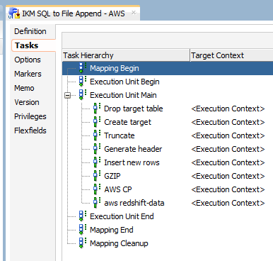
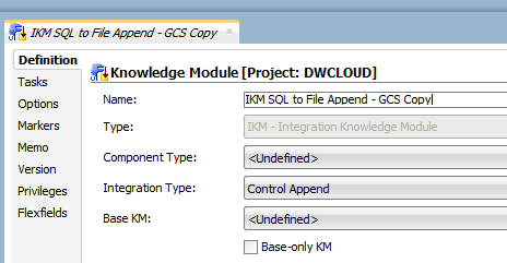
Second step is to create a copy of the current “IKM SQL to File Append” and give it a new name, in my case its “IKM SQL to File Append – Snowflake PUT”. Delete some steps of it and leave only the ones below:

These ones will basically just create a file in a server. This file needs to have the same name as the table that you will want to load in Snowflake, plus the “.txt” extension (e.g., if you are loading CLIENTS table, you need to create CLIENTS.txt file in the server). The target Datastore definition may be anything you want, but I’m following this pattern:

Now you need to add only two more steps in the KM, as below:

Snowflake PUT

The target command is the following:

OdiOSCommand "-OUT_FILE=<%=odiRef.getTable("TARG_NAME")%>_put.log" "-ERR_FILE=<%=odiRef.getTable("TARG_NAME")%>_put.err"

snowsql -c #P_CONNECTION_NAME -w #P_SNOW_WAREHOUSE -r #P_SNOW_ROLE -d #P_SNOW_DATABASE -s #P_SNOW_SCHEMA -q 'PUT file://<%=odiRef.getTable("TARG_NAME")%>.txt @#P_STAGE_NAME auto_compress=#P_AUTO_COMPRESS parallel=#P_PUT_PARALLEL'

We can see that it is basically one OS command that is calling snowsql client. It is passing all the connection information in order to login and then it is issuing a PUT command to Snowflake. This PUT command is sending a text file to a stage area, with auto compress and a defined number of parallel workers. If you are familiar with ODI, you know that all of those # variables need to come from some place. You may implement in any way you want, but in my case, I did put a SQL statement in the command on source tab that returns all this information from a parameter table that is located in the on-premises database, like below:

I even added a CONFIG_CODE filter (which is a KM option that I added to this new KM), in the case of having multiple Snowflake configurations (which is very common to have). So, if you have multiple configs, you may add this option on your new KM and use it when you are creating a new mapping.

Snowflake Copy

This step is very similar to the one before. In the target tab we will have the following:

OdiOSCommand "-OUT_FILE=<%=odiRef.getTable("TARG_NAME")%>_copy.log" "-ERR_FILE=<%=odiRef.getTable("TARG_NAME")%>_copy.err"

snowsql -c #P_CONNECTION_NAME -w #P_SNOW_WAREHOUSE -r #P_SNOW_ROLE -d #P_SNOW_DATABASE -s #P_SNOW_SCHEMA -q 'copy into #P_SNOW_DATABASE.#P_SNOW_SCHEMA.<%=odiRef.getTargetTable("TABLE_NAME")%> from  @#P_STAGE_NAME/<%=odiRef.getTargetTable("TABLE_NAME")%>.txt.gz'

This one is issuing a copy from Snowflake stage to the final table. On the source tab, we have the same SQL shown on the prior step:

And that’s it. You are ready to push data from on-premises to Snowflake in a very fast way. It gives you some work upfront, but I may guarantee to you that it’s worth it.

Thanks, see you soon!

ODI in the hybrid database world – Snowflake JDBC

Posted in Uncategorized on April 13, 2022 by Rodrigo Radtke de Souza

This second post will talk about Snowflake integration with ODI. Let’s picture a scenario like the last post: your company has a large on-premises ETL/database footprint, but it is starting to move slowly to the cloud, in this case, Snowflake. You want to use the existing ODI architecture for this task, but Snowflake is not a technology that comes out of the box with ODI, so how could you do that? Let’s figure it out in this post.

Luckily a good friend of mine, Michael Rainey, wrote about it in his post here. I won’t go over the details because I don’t want to copy and paste what is already written there, but in a very resumed way you need to download the Snowflake JDBC driver, add it to the ODI agent, create/copy a new technology for Snowflake usage and that’s it. It will work just fine.

However, after working with it for some time, I found some details that I think its worth sharing with you. First, differently from the first post where Oracle is already a technology that ODI knows, Snowflake is not and for that reason you may start to face some small issues here and there regarding SQL statements for example. If the KMs or procedures that you are using are standard/universal SQL that both Oracle and Snowflake understands, it will work just fine. If the SQL is kind of different in Snowflake (meaning a different syntax) or it is Oracle exclusive, than you will need to start doing some customizations.  Luckily, most of these customizations should be very simple to adapt to Snowflake.

Another thing is data volume. For small workloads, it works well. For larger ones you will need to do some tweaks. One way to decrease the time loads is by playing with Array Fetch/Batch Update Sizes and Degree of Parallelism for Target, as you can see below.

Array Fetch/Batch Update Sizes are very hard to fine tune to an optimal value, since it depends on a lot of factors like length and size of the table, network, and so on. Sometimes you may fine tune for smaller tables, but larger tables suffer and vice versa. You will need to run some tests and see what the best value for your case is. However, Degree of Parallelism for Target is one that you may increase up to 20 without too much worry and you will see a huge gain. You cannot increase further because Snowflake (at least in my account) has a limit of 20 parallel threads working on the same object at a time.

If you want to see what is happening on the push of data to Snowflake, you may check the Load task of it in Operator and click on Details. It will show you the details and times that each thread took to execute it:

However, even with those tweaks in the Topology, I found myself into situations where the data load was just not fast enough. Upon doing some research and some testing, I figure out that there is a way to push data to Snowflake way faster than JDBC, and it is by using SnowSQL client. This one I’ll cover on the next post.

See you soon!