Archive for the ODI Category

Building dynamic ODI code using Java variables – Table to File example

Posted in ODI with tags , on March 23, 2023 by Rodrigo Radtke de Souza

Written on March 23, 2023 by Rodrigo Radtke de Souza

Hi all. Today’s post is an “enhancement” of one post that I did a long time ago regarding using Oracle’s metadata to build dynamic code. I say it is an enhancement because that technique would use the source/target command tabs and it has a 4000 character limitation. So, if you are trying to build some metadata information that crosses this limit, it will fail.

You should be good using source/target command technique in 90% of your data loads, but there are a few exceptions that we need to go beyond 4000 characters. One of these examples is when you are trying to build dynamic code to generate text file loads in ODI. The example that I’ll show here is about dumping the data from any Oracle table to a text file dynamically, using only one ODI procedure.

This is what we will build. I’ll go over each step in detail:

Basically, it is an ODI procedure that will receive a table name as a parameter and it will write that table data into a text file using pipe “|” as delimiters. This is a very small but useful procedure that you may use when you need to create fast text files from tables/views without going through all the work to create ODI mappings for it.You will need two Logical Schemas, one for the source table and another one for the target file. In this example I used LOCAL_SOURCE that points to an Oracle database and OUTPUT_FILE that points to a folder where the text file will be created.First step is to get the file metadata. As I said, this will be done in a different way now. Instead of using source/target tab commands, we will use Java BeanShell to retrieve this information. This is because ODI creates a very lengthy metadata for each column and the total amount of metadata often crosses the 4000 characters limit. Just as an example, each column in a file text load looks similar to this:

"CRDWG_COLSNP$CRCOL_NAME="+metaDataSrc.getColumnName(i) + "SNP$CRTYPE_NAME=STRINGSNP$CRORDER="+i+"SNP$CRLENGTH=4000SNP$CRPRECISION=4000SNP$CRACTION_ON_ERROR=NULLSNP$"

Here is the full code for the “Get File Metadata” step:

<@
import java.sql.*;

String table_name = "#DWCLOUD.L_TABLE_NAME";
String folder_path = odiRef.getSchemaName("OUTPUT_FILE","D")+"/"+table_name;
String folder_path_txt = folder_path+".txt";
String table_schema = odiRef.getSchemaName("LOCAL_SOURCE","D");
String table_metadata = "/*$$SNPS_START_KEYSNP$CRDWG_TABLESNP$CRTABLE_NAME="+table_name+"SNP$CRLOAD_FILE="+folder_path_txt+"SNP$CRFILE_FORMAT=DSNP$CRFILE_SEP_FIELD=0x007cSNP$CRFILE_SEP_LINE=0x000D0x000ASNP$CRFILE_FIRST_ROW=1SNP$CRFILE_ENC_FIELD=SNP$CRFILE_DEC_SEP=SNP$CRSNP$";
String table_header = "";
String table_header_parameter = "";

Connection ConSrc = DriverManager.getConnection("<%=odiRef.getInfo("SRC_JAVA_URL")%>","<%=odiRef.getInfo("SRC_USER_NAME")%>",odiRef.getInfo("SRC_PASS"));
Statement stmtSrc = ConSrc.createStatement();
ResultSet querySrc =  stmtSrc.executeQuery("select /*+ parallel(64) */ * from "+ table_schema +"." + table_name + " where 1=2");
ResultSetMetaData metaDataSrc = querySrc.getMetaData();

int count = metaDataSrc.getColumnCount();
for (int i=1; i<=count; i++)
  {
	table_metadata = table_metadata + "CRDWG_COLSNP$CRCOL_NAME="+metaDataSrc.getColumnName(i) + "SNP$CRTYPE_NAME=STRINGSNP$CRORDER="+i+"SNP$CRLENGTH=4000SNP$CRPRECISION=4000SNP$CRACTION_ON_ERROR=NULLSNP$";
	table_header = table_header+metaDataSrc.getColumnName(i);
	table_header_parameter = table_header_parameter+":"+metaDataSrc.getColumnName(i);  
    	 
	if (i==count)
	{
  	table_metadata=table_metadata+"CR$$SNPS_END_KEY*/";
	} else
	{   
  	table_metadata=table_metadata+"CRSNP$";
  	table_header = table_header + ",";
  	table_header_parameter = table_header_parameter + ",";    
	}
  }

ConSrc.close();
@>

How it works? It uses a variable (that you will use in an ODI package later on), to figure out which table it will dump into a file. It actually can be other objects that you can query, like a view. Views are actually great to be used here since you may create any kind of business logic and filters on the view and dump the data to a file when needed. It also uses both logical schemas (source and target) to figure out where to read the source data and place the target file.

It then creates a connection object using the source connection that you set in the ODI procedure (please pay close attention to each source/target logical schema in the ODI procedure) and it runs a query where 1=2 just to retrieve the table/view metadata.

Having this metadata in the result set, it loops through it and starts to “build” the dynamic code for the header and the columns. It does some special conditions when it reaches the last column and then it closes the connection.

It may sound complicated, but it’s fairly simple. In less than 40 lines of code we are able to retrieve all metadata to dump any table’s data to a flat file in a dynamic way. The other steps are now very straight forward.

“Create File” step will be as simple as this:

create table "<@=folder_path@>"
<@=table_metadata@>

Same for “Truncate File”:

truncate table "<@=folder_path@>"
<@=table_metadata@>

“Create Header”:

create header (<@=table_header@>)
<@=table_metadata@>

“Insert Rows” is the only one that needs two steps. In Source Command we have:

select     
    /*+ parallel(64) */ <@=table_header@>
from    <@=table_schema@>.<@=table_name@>
where    
    (1=1)    

This one is used to read the source table. In Target Command we have the insert statement to the file object:

insert into "<@=folder_path@>"
(
	<@=table_header@>
)
values 
(
	<@=table_header_parameter@>
)
<@=table_metadata@>
  

Add this procedure in an ODI package, alongside with the ODI variable for the table name:

Add the table/view object that you want to dump the records. In this example, I used a table named SAMPLE_DATA. When I executed the package, I have the following:

If I go to the folder path defined in OUTPUT_FILE logical schema, I can see the data file created there (they are all fake/random rows, not real people information):

I hope you liked this post. See you soon!

Advertisement

ODI Hidden Gems – SNP tables: Query to get load plan execution steps

Posted in ODI, Query with tags , on December 6, 2022 by Rodrigo Radtke de Souza

Hi all,

Today is a short post, but very useful. I often get asked about how to write SNP table queries to get some information from ODI repositories. I posted one about “executed code” here. Today, this is another example of how to get a load plan execution steps that were executed. This one I use in the end of every load plan execution, so it creates a mini report of how each step performed in that load plan. This is useful for ODI Operators, so they can do some analysis of how well their jobs are doing.

This query was created using ODI 12.2.1.4.

WITH 
LP_STEPS AS (
SELECT SLS.I_LOAD_PLAN
     , LP.LOAD_PLAN_NAME
     , I.I_LP_INST
     , SLS.LP_STEP_NAME
     , SLS.I_LP_STEP
     , SLS.PAR_I_LP_STEP
     , SLS.STEP_ORDER
     , LEVEL AS LEVEL_
     , SYS_CONNECT_BY_PATH(SLS.LP_STEP_NAME, ' -> ') AS STEP_NAME_PATH
     , SYS_CONNECT_BY_PATH(SLS.STEP_ORDER, ' ') AS STEP_ORDER_PATH
     , SYS_CONNECT_BY_PATH(SLS.IND_ENABLED, ' ') AS IND_ENABLED_PATH
     , SYS_CONNECT_BY_PATH(DECODE(SLS.LP_STEP_TYPE, 'EX', 1, 0), ' ') AS EXCEPTION_STEP_PATH
     , CONNECT_BY_ISLEAF IS_LEAF
     , SLS.IND_ENABLED
  FROM SNP_LOAD_PLAN LP
    INNER JOIN SNP_LP_STEP SLS
        ON SLS.I_LOAD_PLAN = LP.I_LOAD_PLAN
    INNER JOIN SNP_LP_INST I
        ON SLS.I_LOAD_PLAN = I.I_LOAD_PLAN
        AND I.GLOBAL_ID = '<LOAD_PLAN_INSTANCE_GLOBAL_ID_HERE>'
 CONNECT BY PRIOR SLS.I_LP_STEP = SLS.PAR_I_LP_STEP 
  START WITH SLS.PAR_I_LP_STEP IS NULL
)  
, ALL_ AS (
SELECT L.I_LOAD_PLAN
     , L.LOAD_PLAN_NAME
     , L.I_LP_INST
     , L.LP_STEP_NAME
     , L.I_LP_STEP
     , L.STEP_NAME_PATH
     , L.STEP_ORDER_PATH
     , CASE WHEN L.IND_ENABLED_PATH LIKE '%0%' THEN 'N' ELSE 'Y' END ENABLED
     , MAX(IL.SESS_NO) AS SESS_NO
  FROM LP_STEPS L
    LEFT JOIN SNP_LPI_STEP_LOG IL
        ON L.I_LP_INST = IL.I_LP_INST
        AND L.I_LP_STEP = IL.I_LP_STEP
 WHERE 1 = 1
   AND L.IS_LEAF  = 1
   AND EXCEPTION_STEP_PATH NOT LIKE '%1%'
 GROUP BY L.I_LOAD_PLAN
        , L.LOAD_PLAN_NAME
        , L.I_LP_INST
        , L.LP_STEP_NAME
        , L.I_LP_STEP
        , L.STEP_NAME_PATH
        , L.STEP_ORDER_PATH 
        , L.IND_ENABLED_PATH
) 
SELECT A.I_LOAD_PLAN
     , A.I_LP_STEP
     , A.LOAD_PLAN_NAME
     , A.LP_STEP_NAME
     , A.STEP_NAME_PATH
     , A.SESS_NO
     , CASE WHEN A.ENABLED = 'N' THEN 'Step has been disabled'
            WHEN A.SESS_NO IS NULL THEN 'Step did not run'
            WHEN S.SESS_STATUS = 'D' THEN 'Step finished successfully'
            WHEN S.SESS_STATUS = 'E' THEN 'Step failed'
            WHEN S.SESS_STATUS = 'W' THEN 'Step finished with warnings'
            ELSE 'Other status not relevant'
        END STATUS
     , TO_CHAR(S.SESS_BEG, 'DD-MON-YYYY HH24:MI:SS') AS SESS_BEG
     , TO_CHAR(S.SESS_END, 'DD-MON-YYYY HH24:MI:SS') AS SESS_END
     , S.SESS_DUR
     , REPLACE(REPLACE(REPLACE(SUBSTR(S.ERROR_MESSAGE, 1, INSTR(S.ERROR_MESSAGE, CHR(9) || 'at ')), CHR(10), ' '), CHR(13), ' '), CHR(9), ' ') AS ERROR_MESSAGE
  FROM ALL_ A
    LEFT JOIN SNP_SESSION S
        ON A.SESS_NO = S.SESS_NO
 ORDER BY A.STEP_ORDER_PATH;

I hope you like it! See you soon!

ODI in the hybrid database world – Google BigQuery – gsutil + bq

Posted in BigQuery, Cloud, Google, ODI with tags , , on December 5, 2022 by Rodrigo Radtke de Souza

As we saw in our last post, ODI + BigQuery + Simba Jdbc didn’t give us the performance that we were expecting. But we may apply the same concept that we did for Snowflake: we may create a file, zip it (using GZIP), send it to a storage location (using gsutil) and load it into a table (using bq). Luckily, this is easy to do in ODI and Bigquery. First, we will need to install Google Cloud CLI, which will enable you to use both gsutil and bq. You may read about it here.

Next, we will follow the same steps that we did for Snowflake, first we will create a copy of an existing IKM. In this case, I duplicated IKM SQL to File Append and gave it a new name:

On Tasks, I left some original ones (which will create a text file for us) and I created three new steps: GZIP, Copy and Load.

The first new step is GZIP, because we want to compress our file before moving it to the cloud. Google BigQuery may load zipped files directly from Cloud Storage, but they need to be in a GZIP format. So, on “Target Command” I added this:

OdiOSCommand "-OUT_FILE=<%=odiRef.getTable("TARG_NAME")%>_zip.log" "-ERR_FILE=<%=odiRef.getTable("TARG_NAME")%>_zip.err"

"C:\Program Files\7-Zip\7z.exe" a "<%=odiRef.getTable("TARG_NAME")%>.GZ" "<%=odiRef.getTable("TARG_NAME")%>.txt"

For the sake of simplicity in this example, the path is hardcoded, but in a real-world project, we would make this path dynamic.

Second one is GCS Copy. In this step, we will call “gsutil cp” command that will get a file (in this case GZIP file that we created in the previous step) and send it to a bucket in Google Cloud Storage:

OdiOSCommand "-OUT_FILE=<%=odiRef.getTable("TARG_NAME")%>_cp.log" "-ERR_FILE=<%=odiRef.getTable("TARG_NAME")%>_cp.err"
gsutil cp "<%=odiRef.getTable("TARG_NAME")%>.GZ" gs://<YOUR_GCS_BUCKET_NAME_HERE>

Last step is using “bq load” command that will get the file that is stored in your bucket and load it to a table in BigQuery:

OdiOSCommand "-OUT_FILE=<%=odiRef.getTable("TARG_NAME")%>_bq.log" "-ERR_FILE=<%=odiRef.getTable("TARG_NAME")%>_bq.err"
echo bq load --source_format=CSV --skip_leading_rows=1 --field_delimiter="|" GOOGLE_TARGET.SAMPLE_DATA gs:// <YOUR_GCS_BUCKET_NAME_HERE>/SAMPLE_DATA.GZ| C:\WINDOWS\system32\cmd.exe /k ""C:\Users\<YOUR_USER>\AppData\Local\Google\Cloud SDK\cloud_env.bat""

This command is a little messy, but it works. In your project you may do something more elaborate, but for the sake of this example, it will work. Basically, I’m using the echo trick to call two command lines at once. The first one I run “cloud_env.bat”, which will set my cloud environment variables (this comes with Google CLI installation). Then, I call “bq load”, passing as parameters the source format, the number of heading lines and the field delimiter. In this case, we are using pipe “|” as our column delimiter. After that we pass which Dataset/Table we want to load and from which file (in this case our GZ file).

Seems complicated at first, but the data load speed is worth it. And since all this is in an IKM, you will do it once and reuse it repeatedly.

Before we create a mapping, we need to remember that now we won’t be loading BigQuery directly, but instead we will be loading a text file first. So, we need to create a new model pointing to a File logical schema that will be used to hold our temporary files. For this example, I’ve created a delimited file using pipe and with header. For the columns, I created all of them as Strings.

Now we may create our mapping. In this case, its pretty simple. We just add our Oracle source table and our File target table.

When we execute it, we can see that I was able to load 1,077,500 rows in 76 seconds. Not bad at all:

Once again, we saw that working with files and command line tools were way faster than JDBC connections. Also, if you think a little bit about it, it has other cool benefits. If you threat all your cloud integrations as file transfers, you may create an architecture that can be used across multiple cloud vendors. Your on-premises output will always be compressed files that will be loaded to cloud systems using different ODI Knowledge modules, one for each vendor. Since all of it are text files, ODI mappings may be used to create all sorts of complex logic using your on-premises database as staging and then only pushing the result to the cloud.

I hope you have enjoyed. See you soon!

ODI in the hybrid database world – Google BigQuery – Simba JDBC

Posted in BigQuery, Cloud, ODI with tags , on November 23, 2022 by Rodrigo Radtke de Souza

Hi all! Continuing our series, today we will talk about how to load data into BigQuery using ODI. There will be two posts, one talking about Simba JDBC and another one talking about Google Cloud SDK Shell. You will notice that the first approach (using Simba JDBC) has a lot of challenges, but I think its worth looking at it, so you have options (or at least know why you should avoid it).

First, you need to download Simba JDBC and add it to your ODI client/agent (like what was done with Snowflake JDBC here). Also, you need to “duplicate” one ODI technology (I used Oracle in this example) and name it as BigQuery:

In JDBC Driver, you will add the Simba driver and in URL you will add your connection to Google BigQuery. I’ll not go over the details here, since there are a lot of ways for you to create this URL, but you may check all the ways to create it in this link.

Press “Test Connection” to see if it is all working as expected:

Create a new Physical schema and give it the name of your BigQuery Dataset:

Create a new Logical Schema and a Model. If all is correct, you will be able to Reverse Engineer as you normally do with other technologies:

Let’s go ahead and just create a new mapping. This is a simple one: getting data from an Oracle database and loading it to BigQuery:

As LKM, I’m using LKM SQL to SQL:

As IKM, I just used a Global one:

When I ran it, it fails. If we check Operator, we will see that it couldn’t insert new rows because it was not able to create the C$ temporary table. If we look further, we see that it considers “$” as an illegal character in BigQuery tables:

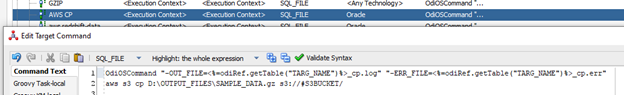
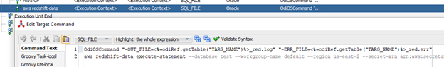
If we get the create table statement from ODI Operator and try to execute in BigQuery, we will see a lot of issues with that:

First, as I said before, we cannot have $ signs, so let’s try to remove it:

It also does not accept NULL. Removing them gave another error:

Varchar2 is not a thing in BigQuery, so if we change it to String, it will work fine:

So, just for us to create a temporary C$ tables, we had to do several changes to it. It means that ODI/BigQuery integration is not straightforward as we did for Oracle Cloud or Snowflake. We will have to do some changes and additions to BigQuery technology in ODI. Let’s start with $ signs. Double click BigQuery and go to Advanced tab. There, lets remove the $ sign from temporary tables (I removed only in C$ for this example):

Also, you need to remove the DDL Null Keyword:

You may need to do way more changes depending on what you need to load, but for this example, we will try to keep as simple as possible.

Next step is to create a String Datatype. You may go to BigQuery technology and duplicate and existing Datatype. For this example, I used Varchar2. Then I changed the Name/Code/Reverse Code/Create table syntax/Writable Datatype syntax.

Another step is to change our source technology, in this case Oracle. We need to do that because ODI needs to know what to do when converting one datatype from one technology to another. We do this by going to Oracle Technology and double clicking in each source datatype that we have and what they compare to the new target technology (BigData). For this example, we will only be getting Varchar2 columns to String columns, so we will just make one change. In a real-world scenario, you would need to change all the ones that you use. Double click Oracle’s VARCHAR2 Datatype, click on “Converted To” tab and select String on BigQuery Technology.

One last change is to go to our BigQuery datastore and change the column types to String:

This should be enough for us to test the interface again. When we run it, no error happens this time:

However, the data load takes forever to complete (I cancelled after some hours trying to run a 1 M rows table). The ODI job was able to create the work table and I could see data flowing in BigQuery, but the speed was just too slow:

I tried to change the Array Fetch/Batch Update size/Parallelism in the Google BigQuery Data Server ODI object, but none of the values that I tried seemed to work fast as I wish:

Not sure if the slowness was due to something in my architecture, but at this point I just thought that, even if worked reasonably fast, it wouldn’t be as fast as creating a file and send it directly to BigQuery (similarly on what we did for Snowflake). Also, the amount of customization is so high to load a simple table, that I really don’t want to think on how bad it will get when we get to some complex mappings.

Not surprisingly, my tests with text files were extremely fast and the customizations needed are minimum compared to the JDBC method, so that’s what we will be covering in the next post.

Thanks! See you soon!

How to use your existing ODI on premise to seamlessly integrate PBCS (Part 3: Inbound Jobs)

Posted in Cloud, EPM Automate, ODI, PBCS, Uncategorized with tags , , on March 18, 2021 by RZGiampaoli

Hey guys, how are you? Continuing the how to integrate PBCS seamlessly using you existing ODI environment series (Part 2 Here), today we’ll talk about Inbound Jobs.

We already know that we’ll need 4 type of jobs for our integration then let’s see what we need to do to create an Inbound Job:

The first thing we need to do is to set the location as inbox (or outbox in case of an extract). This is what enables the button save as a job. If you choose Local, it enables you to run just for one time.

Second, source type. We have 2 choices there, Essbase and Planning. Essbase has the same format that we are used with Essbase exports, the problem is that if we select Essbase we’ll need to have one job per Plan type.

Planning in the other hand has a special format that is very handy for create dynamic objects in ODI as we can see in the table below:

As we can see, the planning format has a column for the account, then the periods, a POV column and the data load cube name (plan type).

The periods on the column is already a nice thing to have since will be way fester to load and way more optimized since we’ll have one how for the entire year.

Of course, this will only be true when we are talking about forecast because actuals normally, we load just one month per time… even so I prefer this format then have one column for the period and another for data.

The POV is also nice because doesn’t matter how many dimensions we have in one plan type, everything will be in the same column, then for integrate is simple since we just need to concatenate all columns but accounts in one column. I recommend using Regular expression and LISTAGG to do so (best function ever for dynamic components).

And to end we need to inform to each plan type that data will be loaded, very nice, you can load all your plan types at once. One job, one file and everything can be done by one generic component in ODI.

After that we need to choose the delimiter used in the file, in this case, I choose pipeline because it’s very hard to have this character in the middle of any metadata.

Finally, we just need to inform the name of the file. That’s all we need to create a job that we can call using EPMAutomate anytime we need it.

ODI Hidden Gems – Unique temporary object names

Posted in Gems, ODI, Tips and Tricks with tags , , on March 11, 2021 by Rodrigo Radtke de Souza

Hi all, I was not going to write about this one because I thought that this “hidden” gem was already known to every single ODI 12 developer out there, but I still get questions on why sometimes some specific data loads fails when they run in parallel, and they work fine when they run in serial. Most of the times, those are related to how ODI handles the temporary objects that it creates to do ETL (like C$, I$, E$ tables).

Let us see one example, which is the default in ODI. I have created one very simple mapping that has one source and one target table.

This mapping is loading data from two databases that resides in different data servers, so it will need to create a C$ table to be able to transfer the data. If we look at ODI Operator, we will notice the following:

The C$ table that it created is named as C$_0SECTIONTYPE. By default, ODI will create this name based on the source component that the data was generated from, so in this case it was a table called SECTIONTYPE. The “0” in front of it is an incremental number that would increase if you had another source with the same name in the mapping. For example, if you had SECTIONTYPE mapped twice as source tables, one would be loaded as C$_0SECTIONTYPE and the other C$_1SECTIONTYPE. ODI does that so we do not have a clash between names within the same ODI mapping.

However, what would happen if you tried to run the same mapping or another mapping that also contains SECTIONTYPE as source at the same time? As you may imagine, one mapping would interfere in the other, since both C$ tables would be called C$_0SECTIONTYPE and both mappings would be trying to load/read/drop it at the same time, which would cause a failure (in a good scenario) or wrong data (in a bad scenario).

To avoid this kind of issue to happen, ODI 10/11 developers were very creative in the past and would create some Java variables and some tweaks in some ODI KMs to make the temp table names dynamic. However, ODI 12 introduces something way simpler to handle this kind of situation, however, its not default and it is kind of “hidden”. If you go back to the mapping, click on the Physical tab, and scroll all the way down. You will notice a check box that says “Use Unique Temporary Object Names” that is unchecked. If you check this one and run it again, you will see the difference.

ODI now created a table named C$_0SECTIONTYPEAIHLNQMAVPK7Q1FR66UM225DF3, which is totally unique, and it will never clash with another mapping running in parallel. But then, another question arises: should I go to each mapping to check this option, if I want all to be unique? Well, the answer is no. There is another “hidden” gem that you can use.

Go to ODI Topology and double click your ODI agent, then go to Properties.

Luckily, you may enable the use of unique temporary objects at an ODI agent level, so you do not need to go back to each mapping and changing them.

That is it for today. See ya!

Essbase Statistics DW: How to automatically administrate Essbase using ODI (Part 8: ODI)

Posted in Essbase, Java, ODI with tags , , on February 19, 2021 by Rodrigo Radtke de Souza

Now its time to glue it all together with ODI. ODI is great here because it can work with different technologies without any effort. In our case, we will run the Java codes that we displayed in this series using Java BeanShell Technology.

Although ODI is great to execute any kind of technology code out there, it does not have a good way for you to write and debug your code while you are developing it. So, I always prefer to create the code in an external Java IDE (like Eclipse), test it and copy the “Main” portion of it into an ODI Procedure.

Another advantage to use ODI is that we can get the connection information from topology itself and reuse everywhere within the package using the command on source/target technique, where you define the connection in the command on source tab and get the information in the command on target tab.

To glue all together in ODI is very simple. We may have all the java codes in one procedure with as many steps as we want (depending in what kind of statistics we want to get, in our case, three). Then we may have another procedure that will hold our pivot queries that we use to transform and load the data into our DW tables. Finally, we may even create our own metrics based on the knowledge that we have from Essbase. Down below is one example of metrics that we may retrieve from the stats that we just gathered.

When we put it all in an ODI package, it will look like this. In this example, we also added a send email component just to inform the users about the job completion.

That’s it folks! Next post will be the last one of this series. Stay tuned!

Essbase Statistics DW: How to automatically administrate Essbase using ODI (Part 7: Essbase DW)

Posted in Essbase, Java, ODI with tags , , on February 17, 2021 by Rodrigo Radtke de Souza

Before we glue it all together in ODI, let us organize the data that we just got from Essbase. In the last post we saw that we gathered all the information we needed inside a generic stage table. Although a generic table is great from an extract perspective, we may decide to split, organize, and load this information in some kind of “historical DW tables” which will help us to analyze the data better over time.

For this series of posts, we have 3 different kind of information: DB Statistics, File Statistics and Outline Statistics. Their structure are very different, so we will generate one historical table for each kind of statistic.

Since we created a generic table to hold all extracted information in rows, now we need to PIVOT the data into columns and load it into the historical tables. This can be easily achieved with a SQL like the one below:

First, we define the columns to be pivoted and use a consolidation function on the data column, like (SUM, AVG, MIN, MAX, COUNT…). Then we specify the data to be pivoted and this data must be a constant in the “IN” clause. Finally, this data is loaded to the DW table using a Control Append approach, since we want to keep adding the current statistics to a historical table for an analysis over time.

If we follow this approach for all three metrics that we retrieved from Essbase, we will end up with three DW tables, like the ones below:

File statistics:

Outline statistics:

DB statistics:

That is all for today! See you!

Essbase Statistics DW: How to automatically administrate Essbase using ODI (Part 6: Java codes)

Posted in Essbase, Java, ODI with tags , , on February 9, 2021 by Rodrigo Radtke de Souza

Hi all, let us demonstrate some examples of Java codes that you may use to retrieve statistics out of Essbase. Since we want to store those stats in an Oracle table, let us begin with an example of how to connect to an Oracle DB, which is simple, as we just need the DB URL, username, and password. Below is how we may create the connection. We also have a prepare statement that we will use to do inserts in our Oracle table.

Since we have a generic table, we can have just one prepare statement and use it to insert all kind of stats there.

Connecting to Essbase is also easy, the only additional information is that you also need to pass the Provider Service, which may be “Embedded” or by Provider Service. Here we are basically doing a sign in to the provider service and then select the OLAP server that we want to use.

Now let us see the first code to get some cube stats. First, we get all the cubes from all the apps and for each cube we get its properties (which is an array in a Key and a Value format). This information is added to the prepare Statement and executed (inserted) into the DB.

The result will be something like this:

Let us jump to a second example. In Java we can issue any Maxl command using the “IEssMaxlSession” class. The result set contains columns and rows, similar with what we get in EAS. Then we need to loop through the rows and get the columns that we need. This information is also added to the prepare Statement and executed (inserted) into the DB.

The result will be something like below.

The last example is how we can get stats from the Essbase outline. We can get member information using IEssMemberSelection with a custom query or find the member directly in the outline using find member. The results contain a set of members that we may loop and analyze its properties. In this case we decided to categorize the results by its storage type.

Again, the result will be something like the one below.

That is it for today. Next post I will show you how you can glue it all together with ODI. See you soon!

Essbase Statistics DW: How to automatically administrate Essbase using ODI (Part 5: Automating using Java Essbase API)

Posted in Essbase, Java, ODI with tags , , on February 8, 2021 by Rodrigo Radtke de Souza

Hi all! Let us talk now about how we can automate this stat gathering using Java Essbase API. Java is the key technology here since it can easily connect and manipulate Essbase through its API. It also can connect to Oracle Database to store our results, run OS commands and more all in one single code. Java is also great since it may be easily deployed to ODI using Procedures and scheduled using ODI Operator. All in all, combining ODI and Java code creates a powerful and seamlessly integration going beyond the database boundaries.

Let us begin with some Java Essbase API basics. The main goal is to develop one single code that will connect in Essbase, retrieve the statistics information and load that in the Oracle database.

Essbase API is very similar with what we see in EAS, in the sense that the structure of the classes follows the same architecture as in a Essbase server (Server->App->Cube->Otl), which makes it easy to find out what you are looking for when looking at the API documentation.

Since we will store this information in an Oracle table, we will also need to know a little bit about Oracle Java API, but luckily this one is straight forward.

With those two sets of APIs, we are good retrieve all the information that we need from Essbase. Each stat has its own number of columns and metrics, so if we create one table for each kind of structure it will be very tricky to maintain and harder to create any kind of generic code. The best way to extract information is to have just one table where we have the properties in the rows instead of columns, this way we have just one structure for all kind of information, no matter the number of columns that returns and we may create generic code around it. Our final table would look like below.

That is it for this post. Next one I will share some examples on how to connect to Oracle DB, Essbase and how to retrieve some stats out of it. Stay tuned!