OBIEE | DEV EPM

Archive for the OBIEE Category

Fragmented and Aggregated tables in OBIEE using ODI Part 5/5: Setting the OBIEE Repository

Posted in Hacking, OBIEE, ODI, ODI Architecture, Oracle, Oracle Database, Tips and Tricks with tags OBIEE, ODI, ODI Architecture, Oracle, oracle Database on February 13, 2020 by RZGiampaoli

Hey guys, how are you?

Finally, we have arrived in the final chapter of the series Fragmented and Aggregated tables in OBIEE and today we are talking about how to Setting the OBIEE Repository.

Just to make easier for you to navigate in this series, here’s the parts of it:

Creating the tables: I’ll explain the advantages and how you can create the fragmented tables and also how to further improve performance using partitioning and sub partitioning.

Managing the partitions of the Fragmented/Aggregated tables: Here you’ll see how to manage all partitions using ODI.

Populating the Fragmented tables using ODI: Here you’ll find how to create generic components to load all fragmented tables we need to.

Populating the Aggregated tables using ODI: Here you’ll find how to create generic components to load all Aggregated tables we need to.

Setting the OBIEE Repository: Finally, we’ll going to setting up the OBIEE repository to make use of all tables.

This post does not intend to be a step by step how to create an OBIEE repository for beginner or anything like that. My intend is to show the main points that we need to do to make our infrastructure to work in OBIEE. Also, I’m working in OBIEE 12c but this will work in the same way in OBIEE 11 too.

Let’s start then from the beginning. After we import all the tables to our repository the first thing, we need to do is to create the joins between the Dimensions and the Fact tables.

Right now, we have an important point to discuss about constraints. We can have the tables create with Primary Keys and Foreign Keys if you want, as well as not null and any other constraints you wish. The thing is, these things normally impact negatively in the data load times and since we are using ODI, we can have ODI to handle this kind of thing during the data load.

Instead of have a PK or an FK we can have a Flow control in ODI checking the metadata before load it. I always prefer this approach for the simple fact that ODI will generate an E$ table with all fallouts for me automatically, and this is very helpful for debugging.

In my case, I left the table without any constraints or Keys, then the first thing I need to do is to join all our star schema together. Since we have 18 table, all table needs to be joined to all Dimensions in the same way except the Period dimensions.

The Period Dimensions will tell OBIEE what is the set of tables he needs to query. If a user does an analysis in a quarter level, with our design, OBIEE must query only the Quarterly aggregated tables. That’s why we have 3 period dimensions, one for each level of aggregation.

For the DIM_PERIOD (the detailed dimension) we’ll going to join it with all detail Fact tables. As you can see, we joined with 3 “D” tables (BS, Income, PL2) and with the other 3 “E” table (same as before).

For the DIM_PERIOD_MONTH we’ll going to join it with all Monthly Fact tables. As you can see, we joined with 3 “D” tables (in the “M” level) and with the other 3 “E” table (also in the “M” level).

And for the DIM_PERIOD_QUARTER we’ll going to join it with all Monthly Fact tables. As you can see, we joined with 3 “D” tables (in the “Q” level) and with the other 3 “E” table (also in the “Q” level).

This is the first step to make OBIEE work with Aggregated tables. The second and last step we need to do is in the Business layer.

After we finish to join everything (if you have all FK’s in place, you’ll not need to do the joins, OBIEE will load then for you) we can start to do our final settings in the Business layer. In this layer is where we’ll going to tell OBIEE how to behave in front of the aggregate tables and the fragmented tables as well.

First, let’s address the Period Dimension. We’ll drag and drop the more detailed dimension first (DIM_PERIOD) and then we’ll going to drag and drop the other 2 period dimensions on top of the first one. This will create 3 sources in that logical dimension.

If you click in each source, you’ll see that OBIEE will automatically map the columns (By Column Name, then all columns must have the same name [case sensitive]).

As you can see, OBIEE maps the columns available in each dimension, making the Fiscal Quarter column for example, have 3 different sources, one for the DIM_PERIOD_QUARTER, another for the DIM_PERIOD_MONTH and one last one for the DIM_PERIOD.

The next thing we need to do is create a dimension for the DIM_PERIOD logical table. This is the last step needed for OBIEE decide which table it’ll query depending of the analysis created. As I said before, if the user does an analysis at quarter level, OBIEE will know by the DIM_PERIOD dimension and the Table sources that the smaller table to query is the DIM_PERIOD_QUARTER, because it’ll be in the beginning of the Drill path.

OBIEE knows for the design of the drill that the Years level has less members than the Quarter level and so on. That’s how OBIEE defines the aggregate table he’ll query.

The last thing we need to do is in the fact table, and it’ll be done at same time we and in the same place we set the fragmentation content. For the Fact tables we’ll do the same thing as the Period. We’ll drag any Fact table first and then we’ll going to drag all the other 17 tables on top of it like this:

As you can see, we have all sources under the same logical table and in the same way of the DIM_PERIOD, OBIEE will map all columns to the right source. In my case you can see that the Details Sources has more columns than the Aggregated Source (as expected).

At this point is important to point out that OBIEE will always going to try to get the most aggregated table possible but, if an user does an analysis at quarter level but ask for a column that only exists in the Detail table, OBIEE will be obliged to query the detail level and ask the database to aggregate the data for us (making the query slower).

Now, we have only one more thing to do for our architecture to work. We need to define which fragmented table OBIEE will access depending of the Source System and the Account hierarchy name. To do that, we’ll have to add a very simple parameter, that can be very complex if we don’t design well, to the Sources in the fact table.

Inside each Source we have a tab called “Content” and in that table we can specify some very important things:

First, we can/need to specify the Logical level that will be used for each dimension in relation to the fact table. What I mean for that is, for example, for the detail table, every dimension will be using the Detail level of the Dimensions (leaf level) as we can see in the image above. For the Monthly level Fact table, instead of the leaf level, we’ll be using the monthly level of the Period Dimension. That’s the last piece of configuration for the aggregated tables. With this setting OBIEE will know that for that Level of Dimension, he should be using the fact that have the logical level set as Month.

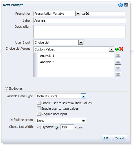
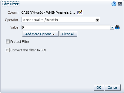
The second important thing we need to set in this tab is the fragmentation filter, and by that we have a field called Fragmentation Content. In this section we’ll going to use a Dimension or more to filter the content. What OBIEE does in this case is, depending of what is selected in the analysis, it’ll select one or more table to query.

For example, in our case we want to, when the Account HIER_NAME is equal to “BS” we want OBIEE to use only the BS tables, if is “INCOME” the use the INCOME tables and lastly if is “PL2” he needs to use the PL2 tables.

It’s nice to know that you don’t need to have the column you want to use in the fact tables, for example, the HIER_NAME column is the highest level of the Account Hierarchy and we don’t have any information regarding this in the fact table. OBIEE just read the Filter and select the right table.

Another very important point about the fragmentation content is that, in cases that you have more than one option, you need to do all possible combinations for that to work properly. For example, if we are doing fragmentation with 2 dimensions, like we are doing, and the dimension A has the values A, B and C and dimension B has values 1, 2 and 3, if the user can select more than 1 value you need to do something like this:

(Dimension A = A and Dimension B = 1) or (Dimension A = A and Dimension B = 2) Or…..

You need to have all possible combinations because in this setting if you say something like Dimension A in (A, B, C) this will only be valid if the user select all 3 values in the dashboard. If he selects just A and B, this filter will not be used.

Then in our case, for simplicity, I had to create an UDA for the Source System otherwise I would have to create all possible combinations between Hier_Name and Source System. Then In my DIM_SOURCE_SYSTEM I have something Like this:

As you can see, the UDA split my Source Systems in the same way I split the data in the table. In the E tables I have just EMC data and in the D tables I have DELL, DTC and STAT data. This allows me to do a simple filter in the Fragmentation Content filter making our lives way easier.

The third important thing is that, in our case, since we can have in an analysis 2 or more sources at same time, for example, the user can select the Source System Dell and EMC, we need to flag the option “This source should be combined with others at this same level”.

This will make OBIEE ALWAYS create an UNION ALL between at least one D table and one E table, even if the user select just EMC for example, we’ll have the UNION ALL between the same level (Month for example) with the filter Source System = ‘EMC’, making the result set return just EMC data.

If we don’t flag this option, OBIEE will never have 2 fragmented table at same time, and that’s not what we want here.

Then basically we have 3 configurations to do in our 18 sources. Looks a lot but is very simple in the end. I create a color code to try make it easier for us to see all the configurations in our source. Yellow is the configuration regarding the Source System, Green is related with the Account Hier_Name and Red is regarding the level of the aggregated data.

As you can see, we have our 3 configurations combined in our 18 sources.

Period Aggregation:
- For detail Fact table we assign the Leaf level of periods;
- For Month Fact table we assign the Month level of periods;
- For Quarter Fact table we assign the Quarter level of periods;
Account Fragmentation:
- For BS Fact table we filter HIER_NAME = ‘BS’;
- For INCOME Fact table we filter HIER_NAME = ‘INCOME’;
- For PL2 Fact table we filter HIER_NAME = ‘PL2’;
For Source System Fragmentation:
- For EMC Fact tables (E tables) we filter UDA = ‘E’;
- For Dell, DTC and STAT Fact tables (D tables) we filter UDA = ‘D’;

And that’s all we need to do to config OBIEE for this architecture. It’s looks overwhelming but in fact is very simple and very fast to do it, and the performance gains are absurd. With this approach I can query 15 quarter of data in the quarter level in 5 seconds. Billions of data in 5 seconds, it’s a lot.

One thing that I would like to mentioning is that normally in the Business Layer is where I rename all the columns for a more business friendly. In this case I decide to do a little test and I left all the names in the same way it’s in the Physical Layer and decide to create Aliases in the Presentation layer. I did that for 2 very simple reasons, one is that it’s easier to just drag and drop staff from the Physical Layer to the Business Layer if everything has the same name. If things don’t match, he duplicates columns, you need to drag and drop column over column, one by one and it’s a lot of work. Second because I wanted to test if this approach is better than my old one or not.

I don’t have any opinion about that yet and in fact, I could had renaming everything and if I need to expand to 36 table for example, I could rename back the columns, do all the mappings and rename back again, then not sure what’s the best approach on that.

It was way more work to rename stuff in the Presentation Layer because the Rename Wizard doesn’t create aliases, then I had to manually rename column by column then I still not sure about this approach.

And this is the end of our Fragmented and Aggregated tables in OBIEE using ODI. I hope this is helpful and see you in my next post.

4 Comments »

Fragmented and Aggregated tables in OBIEE using ODI Part 4/5: Populating the Aggregated tables

Posted in Hacking, OBIEE, ODI, ODI Architecture, Oracle, Oracle Database, Tips and Tricks, Uncategorized with tags OBIEE, ODI, ODI Architecture, Oracle, oracle Database on February 12, 2020 by RZGiampaoli

Hey guys, how are you?

Continuing the series Fragmented and Aggregated tables in OBIEE using ODI and today we are talking about how to Populating the Aggregated tables using ODI.

Just to make easier for you to navigate in this series, here’s the parts of it:

Creating the tables: I’ll explain the advantages and how you can create the fragmented tables and also how to further improve performance using partitioning and sub partitioning.

Managing the partitions of the Fragmented/Aggregated tables: Here you’ll see how to manage all partitions using ODI.

Populating the Fragmented tables using ODI: Here you’ll find how to create generic components to load all fragmented tables we need to.

Populating the Aggregated tables using ODI: Here you’ll find how to create generic components to load all Aggregated tables we need to.

Setting the OBIEE Repository: Finally, we’ll going to setting up the OBIEE repository to make use of all tables.

Today we are in the final step before we can work in our OBIEE repository to put all these 18 fact tables together. The data load for our Aggregated tables.

The aggregation in fact is a very simple process, we just need to remove all detailed columns we have in the detail fact table and leave just the ID’s columns. After that we just need to reduce the level of the ID of the column we want to aggregate and sum all the data at that new level.

In our case we going to use the PERIOD_ID to do that, because period is the most common choice when we talk about aggregated table and serve well in most of the cases.

And that’s why I design the PERIOD_ID as YYYYQMMDD, because is very simple and easy to manipulate this number to go up or down a period, as well to do range or even transform it back to date. It’s way easier than create a surrogate key or whatever, even if you want to work with SCD.

As you probably already guest by now, we’ll use the command on source and command on target again to do the aggregations, this way we can have only one code to spread the data through out aggregate fact tables.

In the command on source for the monthly level table, we just need a query in the source that return the name of the detailed table plus the name of the monthly table. Since I designed all tables with a specific name pattern, we can easily manipulate the table name to get the month table from the detail table like this:

We don’t need anything fancy here because in the last post we create a proc to call six time the same scenario passing different parameter to it.

One of these parameter is the name of the fact table it needs to be loaded and this information is store in the variable #JAT_TABLE_NAME (already replaced by the value in the picture) and what I have done there is just split the table name using REGEXP to get the forth and the fifth occurrences of ‘_’ and concatenate everything back adding a _M_ in the middle of it, creating my Monthly level fact table name.

With data we have the detail table name that the scenario needs to load and also the monthly level fact table name that we need to use for that loop. We just need to create a query to aggregate the data, what’s very straight forward.

As the query will change depending of the design of the table, this one is just intended for explain what needs to be done since the idea is very simple. First we replace the name of the table that we wish to insert data and the table that we wish to get the data from for our to variables: #JAT_TABLE_NAME that we are sending when we call this scenario and #JAT_M_TABLE_NAME that we just create in the Command on Source tab.

With this, for each loop, the scenario will get the data from the right source table and will insert in the right aggregated table. Now we need to aggregate the data, also a very simple matter. All we need to do is to join the detailed fact table with the period dimension and, because this is a range partition, we need to get the first date of that month and the last date of that month, that’s why we have that MIN and MAX filtered by the Year and Month.

With the right data filtered, we just need to aggregate the data and use the FISCAL_MONTH_ID instead of the PERIOD_ID, this way the data will be aggregated by month. And we are done here.

By the way, we could instead of using the between to get the right range of the partition filtered the partition itself using explicit partition filtering:

This will make oracle to go straight to that partition. The only thing is that you need to pass the partition name, that in our case is very straight forward, specially because we are creating and managing the partitions ourselves. We could have oracle create the partitions automatically using INTERVAL (for another post) but if we do that oracle will also create the names of partitions like SYS###### and that will make everything harder to filter by partitions. Anyway, this is just another option we can have.

For the quarter level it’s even easier because we don’t need to worry about range partitions anymore. We just need to have our Command on Source return the Monthly level table name and our Quarterly level table name:

As you can see, the query is the same, the only difference is that we insert a ‘_Q_’ in the middle of our string. And for the insert in the Target Command tab we just need, as before, replace the tables using the right variable in each case, join with the DIM_PERIOD_MONTH to have the right level of data, filter the Monthly level table using any method and then use the QUARTER_ID to sum the Monthly level data to the Quarterly level data and that’s it.

That’s all we need to do to populate all aggregated table. And we finally have all data populated in our tables and now we can start to create the OBIEE repository. It’s wort to mentioning that if you resume everything that I said until this point, we basically had to:

Create our tables;
Create one procedure to:
- Create the partitions;
- Truncate the partitions before we load data;
- Call and loop the scenario that will load data;
- Drop the old partitions
Create another procedure to:
- Load detail data;
- Load Monthly level data;
- Load Quarterly level data;

What this means is that with just two procedure we can maintain and populate a very complex environment in a very clean way with very little points of failures.

This is a very elegant approach and as I always said, if is too complex and/or difficult, you were doing something wrong. It is just a meter of think about the design first, all that needs to be done, and split it in a logical and reusable way. If you do that, everything will be simple to be archived using ODI.

I hope this series has been useful so far and I see you in the last chapter.

4 Comments »

Fragmented and Aggregated tables in OBIEE using ODI Part 3/5: Populating the Fragmented tables

Posted in ACE, Data Warehouse, Hacking, OBIEE, ODI, ODI Architecture, Oracle, Oracle Database, Query, SQL with tags OBIEE, ODI, ODI Architecture, Oracle, oracle Database on February 11, 2020 by RZGiampaoli

Hey guys, how are you?

Continuing the series Fragmented and Aggregated tables in OBIEE using ODI and today we are talking about how to Populating the Fragmented tables using ODI.

Just to make easier for you to navigate in this series, here’s the parts of it:

Creating the tables: I’ll explain the advantages and how you can create the fragmented tables and also how to further improve performance using partitioning and sub partitioning.

Managing the partitions of the Fragmented/Aggregated tables: Here you’ll see how to manage all partitions using ODI.

Populating the Fragmented tables using ODI: Here you’ll find how to create generic components to load all fragmented tables we need to.

Populating the Aggregated tables using ODI: Here you’ll find how to create generic components to load all Aggregated tables we need to.

Setting the OBIEE Repository: Finally, we’ll going to setting up the OBIEE repository to make use of all tables.

In my previous posts we had design our 18 tables and the partition management process. Now we’ll talk about how we’ll going to load data to our fragmented tables. As you can imagine, for the 6 fragmented tables, the code will be the same, the only difference is what goes to each table. Then what we need to make ODI to do for us is to dynamically filter and load the data that comes from the same query to different tables based in a rule.

If you are following this series from the beginning, you probably already guessed what we’ll need to do here. The same thing we did for the Partition management process, well, almost the same thing because we’ll going to do something a little bit more optimize for the data load since this is the most time-consuming step.

The main difference between the approach I explained in the previous post is that it loops one Statement by each row that returns from the Source command in SERIAL, that means, we need to wait it to finish for the second loop to start. For the Partition Management that’s ok because everything there is very fast, but for that load we can have something better.

We don’t need and we don’t want to wait for a serial execution because we have one table for each Loop we’ll perform (This is not the case but even if we have only one table, if we have partitions and/or Sub-Partitions, we can Loop the code by the Partition/Sub partition level and load everything in Parallel. The only case we can’t load in parallel is if we have a single table without partition).

In our case we’ll going to loop all the 6 tables load in parallel. To do that, we are going to use the same approach as before but instead of having the ALTER TABLE in the Command on Target, we’ll going to have an OdiStartScen, to call a Scenario multiple times in PARALLEL. Let’s take a look in the Command on Target:

As we can see, the Command on Target contains an ODI tool called OdiStartScen that is used to call a scenario. We have a few parameters there to set how we’ll going to call the scenario and, in this case, the important one is the SYNC_MODE=2, that means it’ll execute everything in parallel (1 is serial). Everything else are variables that we are using to pass information from the Command on Source to the Called scenario.

A quick tip here before we continue, if you want to know how in havens, I have all this setting in mind, for your information I don’t, but there’s a very easy way to find out. Just drop an ODI Start Scen from the ODI Toolbox in any part of your scenario and fill with the information you need:

In the General we set the scenario we want to load, version of the scenario (-1 is always the latest scenario you have), the Synchronous and Asynchronous mode (serial and parallel), Session name, in case you want to have an different name showing in your execution (this is always a good Idea to have since you are looping the same code with different parameters, then in my case I pass as a variable the name of the table, the period and the hierarchy that scenario will be loading).

In the Additional Variables tab you can set all variables you need to use inside the scenario (as you can see in my case, I have a lot of variables because the complexity of my sources, you case will be different).

And after you set everything, you just need to click in the Command tab to get the code that ODI generates based in the setting you did:

This is the code that you need to paste in the Command on target to call a scenario. After that you can delete the OdiStartScen object from your scenario and continue the development. Another advantage of this is that if you have the code and want to create an OdiStartScen step in a scenario, you can paste in the Command tab and the General/Additional Variable will be filled based on the code.

With the Target code ready we just need a query that will going to pass all the information needed to call the scenario. In my case, I pass a lot of information to the target, as you can see by the amount of variable I have. Also, the variable information doesn’t need to come only from the command on source. If you have variable in your scenario and they are the same for all the loops, you can just use these variables to pass their values to the Scenario the command on target is calling. The command on source needs only to have the information that will dynamically change in each loop.

In my case I’m passing all kind of information like the SESSION_NAME (the name of the session that we use to create parameter specific for each session we have and use the same variables for all, more information HERE) but the important one for us is the TABLE_NM.

In my case, the other variables will change the values depending of the table we need to load for each time we loop. To do that I insert all information I need to be pass to the scenario I’m calling in a Parameter table (that I like to call ODI_PARAMETERS). This way I can easily query this table to get specific information I need for each Loop I’m going to perform.

With all this set, we just need to create a child scenario and add “Declare” variables for each Variable we want to pass to the internal scenario like this:

As you can see, this is a very simple scenario that contains just one procedure that’ll be used to load the data to our tables.

This approach can be done with Interfaces as well, in fact with anything at all. We can have a mains scenario that loops a very complex scenario, that loops another scenario and so on. This is a very nice way to loop something because we have a lot of control over this kind of loop as well, we can change the behavior of each loop because the info we get from the Command on Source.

Also, a very good feature is that, if the source query doesn’t return any rows, the Command on Target is not executed at all. Then you’ll always have a clean execution. For example, if you have a folder that can have 0 to X number of files and you want to create an scenario to load it, the best approach would be to read this folder files (OS command to a file and loaf file or Java or Phyton or…) and store the info in our ODI parameter. Then we create a proc to call a scenario that will contain the interface that will load each file, and finally we just do a Select in the Command on Source to get the name of the files in the folder. With that, if we have 0 files, nothing will be executed, but if we have 1000 files, we’ll loop the scenario 1000 times and each time we’ll pass the name of a different file to the internal scenario. Very neat way to do it.

Inside the procedure we just need to create the query need to load the data and use the variables to filter the right data and load the right table. This is not my case but if you have different source for each table you want to load, just insert this information in the parameter table and pass it to the internal scenario. Use these variables to replace the Table Names in the SQL and you are done.

And that’s it. This is all we need to do to load all our 6 fragmented tables. In my next post I’ll be talking about how we can aggregate our data and load our Aggregated tables.

I hope you guys enjoy and see you soon.

4 Comments »

Fragmented and Aggregated tables in OBIEE using ODI Part 2/5: Managing the partitions of Fragmented/Aggregated tables

Posted in OBIEE, ODI, ODI Architecture, Oracle, Oracle Database, Performance, SQL, Tips and Tricks with tags OBIEE, ODI, ODI Architecture, Tips and Tricks on February 10, 2020 by RZGiampaoli

Hey guys, how are you?

Continuing the series Fragmented and Aggregated tables in OBIEE and today we are talking about how to Populating the Fragmented tables using ODI.

Just to make easier for you to navigate in this series, here’s the parts of it:

Creating the tables: I’ll explain the advantages and how you can create the fragmented tables and also how to further improve performance using partitioning and sub partitioning.

Managing the partitions of the Fragmented/Aggregated tables: Here you’ll see how to manage all partitions using ODI.

Populating the Fragmented tables using ODI: Here you’ll find how to create generic components to load all fragmented tables we need to.

Populating the Aggregated tables using ODI: Here you’ll find how to create generic components to load all Aggregated tables we need to.

Setting the OBIEE Repository: Finally, we’ll going to setting up the OBIEE repository to make use of all tables.

In my previous post we design 18 tables and its partitions and sub-partitions. Now what we need to do is to make ODI manage these partitions for us. As I said before, the Sub partitions will be static and if we need to create one more sub-partitions, we’ll be doing that manually. That’s always the best choice because manage sub-partitions add a layer of complicity that is not needed.

With that said, if you need to manage the sub-partitions, you can use the exactly same approach I’ll show here just adapting to the needs of the sub-partition’s creation and sub-partition template update.

Let’s start analyzing what needs to be done. For each table we need to issue this command to the database:

For List partitions:

ALTER TABLE table_name ADD PARTITION partition_name VALUES (value[, value]…);

For Range Partitions:

ALTER TABLE table_name ADD PARTITION partition_name VALUES LESS THAN (value[, value]…);

Sounds hard but in fact is very simple and it’ll going to work in any SQL you have. To do that this we will use a procedure with our ALTER TABLE statement in the Command on target tab and a SELECT in the command on source to pass the information we need to create the partitions like the table names, the partition name and the partition values.

For each row that the SELECT on source returns, the statement in the Command on target will be executed, and we can pass the values from the SELECT in the Command on Source to change the behavior of the statement in the Command on target.

This is something very important that we need to understand about ODI. ODI It’s not an ETL tool but a code generator tool that orchestrate Database and a lot of other tools if you will.

What I mean by that is, until ODI send the code for the database to execute, everything that ODI does is to generate code. If we use the ODI API it’ll replace it before send to the database as well to replaces the variable with their values, meaning a variable like this #SQL on the Command on Target tab could contain an entire dynamically generate INSERT that ODI would replace before send it to the Database.

And this is why ODI is so powerful, because we can manipulate string and make everything dynamic.

Then our query in the source should return something like this:

The query will change depending of your design of the application then I don’t think sharing my query will going to help. One tip I can give you is always compare the name of the partition with the content of the column PARTITION_NAME on ALL_TAB_PARTITIONS view to see if the partition you want to create already exists to prevent an error in ODI, in fact you have 2 choices, either do this or flag the step as Ignore Error to end the step with a warning. I prefer to compare and end the step without warnings, then I compare.

Another thing to notice is that for FY20 Feb, my PARTITION_VALUE (MAX_PERIOD) is the 1 day after the last day of the month. It’s hard to see here because the calendar used by the client is all different but if you have the normal calendar and the mask you have for you PERIOD_ID is YYYYMMDD, for 2020/Feb you partition ID needs to be 20200230 (Feb ends 02/29/2020).

That’s because this is a RANGE partition, and for RANGE partition we define the partition value as VALUES LESS THAN, what means that everything under 20200230 will be FEB unless we have a smaller partition (JAN) below it. But for example, if you smallest partition is 2018/Jan, everything below that period will be inserted in the 2018/Jan partition, then you need be careful with when you’ll start to create partitions.

Another important thing to mention is that you cannot insert a partition smaller than an existing partition, just bigger. That means, if you start with 2018/Jan, it’s impossible to create a 2017 partition, the only way is to drop the table and create the table starting by 2017. A RANGE partition needs to be sequential and always growing.

Having these values returning from the SELECT on the Command on source tab, the only thing that is left is to use these variables in the statement in the command on Target tab like this:

ALTER TABLE #TABLE_NM ADD PARTITION PARTITION_NM VALUES LESS THAN (#MAX_PERIOD);

Pay attention on the values of the partitions. In this case the values are numeric, that is why I’m not using quotes. If the values were String, we need to enclosure the variable with quotes.

And that’s it, this is all we need to do to manage partitions using ODI. Because the SELECT on the source returns All tables with their partitions name and values and we pass to the TARGET statement this information, for each row in the source the target will be looped, creating the partitions you need for each table.

We are done for the fragmented tables. Now we need to manage the partitions for the Aggregated table. The approach is the exactly the same, the only thing that will change is the content of the query from the Command on Source tab and that the PARTITION now will be a LIST Partition instead of a RANGE partition.

We could have done just one query to return all values including if that was a RANGE or a LIST partition, but for the sake of simplicity is always better to split the scenarios to not over complicate something simple.

For the month level we need the query in the Source to return: