Hey guys how are you? Today I’ll continue to talk about the Oracle Always free cloud offering and I’ll try to summarize what you can do after your account is set up. If you want to know how to setup you account you can find it HERE.
After you receive an email saying everything is set you can login in your account and you’ll see a screen like this:
This is the main dashboard. Here’s where you’ll create your Database, your VM’s, convert your account to paid, manage your account, ask for help, etc… Let’s start with the main dashboard:
(1) Quick Actions: Here you’ll find the most important links as quick actions.
(2)Compute: This is where you can create a VM to be used with your databases. You can use it to install tools and develop whatever you want inside the your environment.
(3)Networking: Here’s where you set up your cloud network. This is the first step you must do to ensure your VM and databases will be in the same network and reaching each other.
(4)Autonomous Transaction Processing: This is where you create a transaction database.
(5)Autonomous Data Warehouse: This is where you can create your Data Warehouse database.
(6)Search: A quick way to view all your resources.
(7)Account Center: Here’s a quick place to manage your account and see how many credits you have and billing information
(8)Main Menu: This is the main menu where you have access to everything that you can do inside your Cloud.
(9)Top Bar: Where you can change regions, in case you have more than one region, access the Cloud Shell (for OS commands), see the help, ask for help in the chat, change language and see your profile.
(10)Start Exploring: Here’s a place where you can find articles to help you start setting up your environment.
(11)What’s new: And finally here’s where you can see news about Oracle cloud, like releases and things that will be added.
One important thing to add here is that before you add anything or create anything, look for the “Always Free Eligible” logo or description to be sure you’ll not buying anything by mistake. Now about the main menu:
Core Infrastructure: Here’s where you can set your VM’s, networks and storage options.
Database: Here’s where you can Set your databases options, backups and Servers (VM or Bare metal).
Data and AI: Here’s where you can set your Big Data and AI environment.
Solution and Platform: Here’s where you can set your Analytics cloud services, Integrations, monitoring and marketplace.
More Oracle Cloud Services: Here’s where you have other cloud services.
Governance and Administration: And here is where you can administrate your environment like provisioning security, Account Management, Identity and Governance.
As you can see there’s a lot that can be done, but we’ll concentrate in the “Always Free” content, but the following list summarizes the Oracle Cloud Always Free-eligible resources that you can provision in your tenancy:
Compute (up to two instances)
Autonomous Database (up to two database instances)
Load Balancing (one load balancer)
Block Volume (up to 100 GB total storage)
Object Storage (up to 20 GiB)
Vault (up to 20 keys and up to 150 secrets)
In the next post we’ll setup our environment. See you soon guys.
I decide to do some posts about Oracle Always free offering, how it works, how you setup things, a few things we can do with that and maybe more. I think is fair for us to start by what’s it and what you need to do to get one.
Basically Always Free is a services for anyone that wants to try the world’s first self-driving database and Oracle Cloud Infrastructure for an unlimited time. The ideas is let people explore the full functionality of Oracle Autonomous Database and Oracle Cloud Infrastructure, including Compute VMs, Block and Object Storage, and Load Balancer, all of the essentials for developers to build complete applications on Oracle Cloud.
Oracle’s Free Tier program has two components:
Always Free services, which provide access to Oracle Cloud services for an unlimited time
Free Trial, which provides $300 in credits for 30 days to try additional services and larger shapes
The new Always Free program includes the essentials users need to build and test applications in the cloud: Oracle Autonomous Database, Compute VMs, Block Volumes, Object and Archive Storage, and Load Balancer. Specifications include:
2 Autonomous Databases (Autonomous Data Warehouse or Autonomous Transaction Processing), each with 1 OCPU and 20 GB storage
2 Compute VMs, each with 1/8 OCPU and 1 GB memory
2 Block Volumes, 100 GB total, with up to 5 free backups
10 GB Object Storage, 10 GB Archive Storage, and 50,000/month API requests
1 Load Balancer, 10 Mbps bandwidth
10 TB/month Outbound Data Transfer
500 million ingestion Datapoints and 1 billion Datapoints for Monitoring Service
1 million Notification delivery options per month and 1000 emails per month
Well, if you ask me this is far better than install an Oracle XE in your machine and configure everything there for you to learn or to create some small app. In fact, if you want to learn, it’ll far better if you start learning in an cloud environment since everyday we have more and more companies migrating to cloud.
Ok, but what do you need to do to get one? In fact is very easy, you just need to access this link and click in the Start for Free button. After that you have to fill a short form where you need to inform:
Your email and user information like address and cellphone
You need to validate your cellphone through message (Oracle will send a code to your cell)
You need to choose the region you’ll going to have you OCI (Oracle Cloud Infrastructure)
This needs to be as close as possible as your real region to decrease latency and improve network performance
Some regions are not available for always free (it’s written next to the region name if is available or not)
And you need to add a credit card to your account
You’ll not be charged but you may see 1 Dollar/Euro/… getting charged but it’ll be return
Also, Revolut card don’t work, you need a proper credit card.
And that’s it, Oracle will create your account (in fact takes around 15 minutes until you receive a email with further instructions [Bare in mind that because the COVID-19, it’s taking several days to create a new account]). After you receive your email, you can login in your dashboard and start to create your network, Disk, Database, VM’s and more.
We’ll see how to configure a database in my next post. I hope you enjoy this and see you soon.
Hey guys how are you? I hope you guys are not insane after this 2 months of quarantine. Anyway, is time for us to finish the send email job. In the previous post HERE I explained the Jython code and the HTML code that we need to use to create our HTML table in our email. Today we’ll going to do it become dynamic.
As we saw, for every row we want it we need to have a block of HTML code that will draw the table, color the table and write the content of the cell in our table. We need this to change dynamically if we want to be useful for us, and to do that we need to write a SQL code to create this HTML code for us.
In my case I generate this code here to be my header:
This is saying that I’ll have 16 columns (COLSPAN=”16″) with Center alignment and the name of the table will be “Restatements Control – Group ID: 1” (where the 1 will be dynamically generated as well).
Now we first need to write a query to get this info for us. Since this is a very project related query, I don’t think it’ll do any good for you guys to put my query here, but I’ll explain what I was looking for. First I’m querying the ALL_TAB_PARTITIONS to get all partitions related with that table. Then I was querying a control table that every time the jobs run, it inserts in this table the period loaded, if there’s errors or not, the log folder path and the interface that run the job.
After that I do a FULL OUTER JOIN between this 2 tables to see all partitions I have and how many of these partitions were already executed. Next I PIVOT the information to get a table like data and the results is similar to this:
I created some simple Status code to make easy to manipulate later. NP is “No Partition”, N is “Never Run”, Y is “Warning”, R is “Error” and G is “Success”. Also, when is Y or R I have the Log Path associated with that run, this way the users can click and go to the log folder of that execution.
In my case this is important because this is for an restatement process where the business want to restate the entire past and we have millions of rows per partition, and they want flexibility to run as fit. Then we need to track the executions over time.
Now, the only thing that needs to be done is to convert this information in HTML code. This is easy since we just need to concatenate strings all over the place. Let’s see how I have done it:
The result is one big string for each row the query results. Each column was concatenated with a “Enter” between than, so when this code is used, we’ll have proper indentation for readability. This is the query I used to concatenate everything:
Basically is a lot of DECODE’s to convert my STATUS code in colors and some REGEXP to split the STATUS from the Log path. That’s it for SQL. Now the only problem we have is that this is a very big string and the only way for us to store this is to use a PL/SQL because inside a PL/SQL a Varchar2 (32767 bytes) variable is bigger than inside SQL (4000 bytes).
We just need to create a simple PL/SQL to insert and concatenate all this rows into a CLOB that is a little big bigger (4 GB). To do that we just need to do something like this:
DECLARE

CURSOR C_HTML_TAG IS

	SQL HERE;

V_HTML_BODY CLOB;

BEGIN

    FOR DADOS IN C_HTML_TAG LOOP
      V_HTML_BODY := V_HTML_BODY || TO_CLOB(DADOS.SCRIPT);
    END LOOP;

    INSERT INTO FDM_ODI_RUN.TMP_HTML_BODY_DW (HTML_BODY) VALUES (V_HTML_BODY);

END;
That’s it, now for the easy part, use it in ODI. To do so we’ll have a command in the SOURCE querying the TMP_HTML_BODY table and then we’ll pass #SCRIPT info to our Jython target code:
Hey guys how are you? Today I’ll talk a little bit how can we create a dynamic HTML table email from ODI using Jython.
First of all, let me give you a little bit of context. I had to build an ODI process to restate the past data in our DW. That means, the business wanted, to a certain point in time, to go back all the way to the first period we have in our DW and restate the data based in a map table that they provided.
That’s all right, the biggest problem is that this table is partitioned by Source System and Period, and the business wanted the process to be flexible enough to let them run 1 period and 1 source system at time or to run an range of period and ALL sources at time (and any combination of these 2).
Also all right, my problem now is how to provide the business with a reliable way to tell them what they already run, what is still pending, if we had an error in a period or if there’s some validation fall outs in a period. In other words, how to track the process during execution.
My answer to that, I decide to send a email with a table that shows the source system and years in the rows and the months in the columns, and based in a color code, I paint the cells based in the status of the execution.
This post will be about the Jython/HTML code we wrote and the next post will be about how to make it dynamic in ODI. Let’s start it with the Jython part:
import smtplib

from email.mime.multipart import MIMEMultipart
from email.mime.text import MIMEText

mailFrom = "ODI Services <donotreply@ODI.com>"
mailSend = 'email@here.com'

msg = MIMEMultipart()
msg['Subject'] = "Subject here"
msg['From'] = mailFrom
msg['To'] = mailSend

html =
"""\

HTML CODE HERE

"""

part = MIMEText(html, 'html')
msg.attach(part)
s = smtplib.SMTP('SMTP SERVER HERE')
s.sendmail(mailFrom, mailSend.split(','), msg.as_string())
s.quit()
This is everything you need to have in your procedure to send a HTML code by email. It’s a very simple code, basically we import “smtplib” lib and that will handle the email sending, after that we just need to inform the user, password and SMTP server and use the “sendmail” to send the email. Pretty straight forward.
Now, in the meddle of the code, we have the HTML part that needs to be included. In our case, it’ll be a table. To test the HTML code, you can google “HTML test runner” that it’ll bring a lot of places in the internet where you can run your HTML code and test to see the results. It’s pretty handy, and I’m using this one here.
To create a simple table in HTML we just need this code here:
This code is also fairly simple and basically we have:
<TABLE> tag, where you define the margins, border size, width of the table, cell padding and cell spacing. There’s more options there but you can easily find in the HTML doc.
<TR> tag, where you define the amount of columns using the COLSPAN property as well the alignment of the text there
<TH> tag, where we define the cells of our table itself. There’re a lot of properties for this but I’m using juts a fix 20% width for each cell, just to size them the same (since I have 5 columns), the Color of the cells and the message I want to send.
This is my legend table that will come above my real table, but the configuration is the same in both cases. We’ll have one <TR> block for each line we want to have and as much <TH> lines we need for each cell we want to have. In the end my final table is like this:
As you can see, I send an email with all periods that needs to be restatement showing if the interface already ran, if that was a success, or it had warnings or errors (with the link straight to the error file, if it was not loaded yet and even if we don’t had the partition created for that period/source.
Now, as I said, we need one <TR> per line and, in this case, 16 <TH>, one per cell. As you can imagine, that’s a lot of code that needs to be write there. thanks god I’m using ODI to do that for me, and we’ll take a look on this in the next post.
Just a quick one today, Oracle is offering free access to online learning content and certifications for a broad array of users for Oracle Cloud Infrastructure and Oracle Autonomous Database, and will be available until May 15, 2020.
This is a great opportunity and if you want to learn more, you can find it here.
In case you haven’t already heard about this great opportunity, please click below to learn how you can access *FREE* Oracle Cloud Infrastructure and Oracle Autonomous Database online learning and certifications until May 15th. With all this quarentine stuff going on, its a great opportunity to learn and get certified for FREE on very interesting topics that may benefit a wide range of professionals. This is a great move done by Oracle to increase the number of people with knowledge around its Oracle Cloud products.
Hey guys how are you keeping? I hope everybody is healthy and keep this way in this difficult times.
And to make our life less complicate, here’s another tip. Let’s talk about how to concatenate stuff in Oracle.
Imagine a simple case, we want to query the Planning repository to get the list of UDA’s a member have. We can easily do that by query the HSP_OBJECT, HSP_MEMBER_TO_UDA and HSP_UDA tables.
I’m filtering just 3 products to make it easier for us to see. The results shows that each project has a different number of UDA’s, and we never know how many it’ll be, then the easiest way to concatenate them is to use the command LISTAGG (or WM_CONCAT if you are in a DB version prior to 11.1).
The command is very simple LISTAGG(Column, Separator) WITHIN GROUP (ORDER BY column). As we can see the command allow us to select the separator we want (can be comma or any string really) as well to order the results by another column). Let’s take a look in the example above.
As you can see, it easily create a list split my comma (as specified) for me, and the nice thing about it is that I don’t need to do any string treatment if return null or if I have just one string on it and things like that.
This is an extremely good Function and we heavily use it in ODI to generate dynamic code because its simplicity, for example, we can generate a SQL statement on the fly using the command on source and command on target:
With this results we can easily pass this info to the command on target to generate a dynamic query where ODI will replace the columns we got in the target as well the table name and will also loop for each row we have in the source. This is very handy.
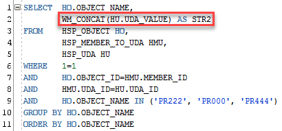
And for the ones that are not in the ORACLE 11.2 and ahead, we can still do that using WM_CONCAT. Is not as powerful as LISTAGG, but works pretty well. Let’s try the first example again:
I cannot show you the results since WM_CONCAT was decommissioned in the 12c (my version), but it’ll work like this. We don’t have the option to choose the separator and to make the string unique and to order by it we need to add DISTINCT in the command WM_CONCAT(DISTINCT column).
Today a quick tip that I think is very useful. From time to time the business ask us to validate if a table has data or not before we load it. It’s fare, specially if you use a truncate and insert approach.
The problem is, sometimes, the table/view they are asking for has millions of rows, and there’s no other safe way to validate if a table has data or not than querying it.
I just fixed a case where an interface had a validation that basically counts 3 different tables that together had 40 million rows per period. This validations were taking around 1000 sec to happens.
The data load that happens before that took 1200 sec. Then, basically the validation process were taking as much time as the load process.
After some changes, the query now is validating the 3 tables in 0.3 seconds. Way better than before. Basically I just used 3 things:
The hint /*+ FIRST_ROWS(1) */ that makes oracle prepare the best plan to query just one row (in my case since I used 1 as parameter.
The filter ROWNUM = 1 to make sure oracle just return 1 row, if we don’t use that, the hint can make everything very slow because oracle will be planning for just one row, but without filtering it’ll bring more (using the best plan possible for 1 row).
And UNION ALL instead of UNION, because there’s a huge difference between them. when you use UNION, oracle matches the sets of data to make sure you have unique rows after that. UNION ALL in other case, just bring everything each set return without any extra process to validate anything. UNION ALL is always faster than UNION.
In the end I have an query like this:
As you can see, the query is very simple and for this example I just had the name of the table there, then we know the table is not empty for that period. We can do other approach like summing then all together and validate if the results is = 3 for example or any other logic we need can be implemented on top of this query.
I hope this is helpful for you guys and see you in the next post.
Today it’ll be a quick tip for you guys that like/need to query the Planning repository.
The Planning repository stores both the Plan Type and the Consolidation in a very particular way, in fact this is true for a lot of other things like security, form properties etc… but I’ll focus these 2, that are the more often used and the solution is the same for all of them anyways.
If we take a look in the HSP_PLAN_TYPE table we’ll have something similar to this (depending in how many plan types you have in your app).
As we can see Planning stores in this table all the plan types that were created when we setup the application. In my case I have 4 plan types and we can have up to 5 BSO plan types in a Planning app. Now, if we join the HSP_OBJECT and the HSP_MEMBER filtering the OBJECT_TYPE = 2 we can take a look in all the dimensions we set in the repository.
The USED_IN columns is the column that says to planning in witch plan type that member will exists. The interesting thing here is that, you don’t see the PLAN_TYPE ID that you supposed to right? And that is because a member can exists in more than 1 plan type right, and if we use the PLAN_TYPE ID straight, we would need one row for each plan type right?
Instead, we have just one row but we also have the ability to tell Planning where that member should exists, and we can do that by summing the PLAN_TYPE ID’s together. In the example above, the Account dimension exists in all 4 plan types (1+2+4+8 = 15). Now the Products dimension exists only in one plan type (1), and by the number you can say that is the Pnl Plan type.
you seen the idea here is to check if a PLAN_TYPE ID exists inside that number we have here in the USED_IN column. Another example is the Employee dimension that has the USED_IN set as 8. The only number that will fit in here is the 8 itself (1+2+4 = 7, 1+8 = 9…) meaning the Plan type is WrkForce.
I think the most used way for us to figure out if a number exists inside another number is to use MOD.
CASE WHEN MOD(USED_IN,2)>=1 THEN 1 ELSE 0 END PT_1
CASE WHEN MOD(USED_IN,4)>=2 THEN 1 ELSE 0 END PT_2
CASE WHEN MOD(USED_IN,8)>=4 THEN 1 ELSE 0 END PT_3
CASE WHEN MOD(USED_IN,16)>=8 THEN 1 ELSE 0 END PT_4
CASE WHEN MOD(USED_IN,32)>=16 THEN 1 ELSE 0 END PT_5
The Oracle MOD(N,M) is used to return the remainder of a dividend divided by a divisor where:
N
Dividend.
M
Divisor.
Pictorial Presentation of MOD() function
Then in our case, we need to test if the USED_IN number contains the PLAN_TYPE ID on it, and for that we need to MOD it by rolling sum of the plan types + 1. To make it easier I’ll put that in numbers:
N = USED_IN = 31 (max number possible)
M = PLAN_TYPE ID = 1 (Pnl) what I want to test) + 1 = 2
MODE (31, 2) = 1
31/2 = 15 Reminder = 1
MOD = 1
What that is telling us is that if the MOD is = 1, the Plan type 1 exists in that number. I run a simulation just to show us when the Plan Type 1 does not exists in the USED_IN:
As we can see, the Plan Type 1 only exists in the odd possible results (as expected) what means in any other possible combination of the other 4 plan types he doesn’t exists (2, 4, 2+4=6, 8, 8+2=10, 8+4=12, 8+2+4=14, 16, 16+2=18, 16+4=20, 16+2+4=22, 16+8=24, 16+8+2=26, 16+8+4=28, 16+8+2+4=30).
The same is true for the other Plan types, you can try then out using the MOD. Now, this work well but there’s a way easier and clean way to do exactly the same thing using the function BITAND.
The BITAND function treats its inputs and its output as vectors of bits, the output is the bitwise AND of the inputs. Basically it performs below steps.
Converts the inputs into binary.
Performs a standard bitwise AND operation on these two strings.
Converts the binary result back into decimal and returns the value.
Ok, it looks more complicated now, but the good news is that to use is simpler than it sounds like. The main difference between this function and MOD is that MOD returns a boolean, BITAND return the value you asked if it’s true. Expanding my previous test using BITAND:
As you can see, with BITAND returning the number you asked for instead of 0 or 1 make it possible for us to Join the HSP_PLAN_TYPE with HSP_MEMBER using the USED_IN and the PLAN_TYPE in the BITAND Function as a Join:
As you can see, this is a far better way to split the members by Plan Type. And now we can see that the Dimension Products only exists in the Plan Type Pnl and that Entity exists in 4 different plan types. We don’t need to worry about any mathematics formula to create all our MODs, we just need to Join our Plan Type table with the BITAND of USED_IN by PLAN_TYPE.
The Consolidation is another place where you can use the exactly same thing. Instead of using something like this:
Finally, we have arrived in the final chapter of the series Fragmented and Aggregated tables in OBIEE and today we are talking about how to Setting the OBIEE Repository.
Just to make easier for you to navigate in this series, here’s the parts of it:
Setting the OBIEE Repository: Finally, we’ll going to setting up the OBIEE repository to make use of all tables.
This post does not intend to be a step by step how to create an OBIEE repository for beginner or anything like that. My intend is to show the main points that we need to do to make our infrastructure to work in OBIEE. Also, I’m working in OBIEE 12c but this will work in the same way in OBIEE 11 too.
Let’s start then from the beginning. After we import all the tables to our repository the first thing, we need to do is to create the joins between the Dimensions and the Fact tables.
Right now, we have an important point to discuss about constraints. We can have the tables create with Primary Keys and Foreign Keys if you want, as well as not null and any other constraints you wish. The thing is, these things normally impact negatively in the data load times and since we are using ODI, we can have ODI to handle this kind of thing during the data load.
Instead of have a PK or an FK we can have a Flow control in ODI checking the metadata before load it. I always prefer this approach for the simple fact that ODI will generate an E$ table with all fallouts for me automatically, and this is very helpful for debugging.
In my case, I left the table without any constraints or Keys, then the first thing I need to do is to join all our star schema together. Since we have 18 table, all table needs to be joined to all Dimensions in the same way except the Period dimensions.
The Period Dimensions will tell OBIEE what is the set of tables he needs to query. If a user does an analysis in a quarter level, with our design, OBIEE must query only the Quarterly aggregated tables. That’s why we have 3 period dimensions, one for each level of aggregation.
For the DIM_PERIOD (the detailed dimension) we’ll going to join it with all detail Fact tables. As you can see, we joined with 3 “D” tables (BS, Income, PL2) and with the other 3 “E” table (same as before).
For the DIM_PERIOD_MONTH we’ll going to join it with all Monthly Fact tables. As you can see, we joined with 3 “D” tables (in the “M” level) and with the other 3 “E” table (also in the “M” level).
And for the DIM_PERIOD_QUARTER we’ll going to join it with all Monthly Fact tables. As you can see, we joined with 3 “D” tables (in the “Q” level) and with the other 3 “E” table (also in the “Q” level).
This is the first step to make OBIEE work with Aggregated tables. The second and last step we need to do is in the Business layer.
After we finish to join everything (if you have all FK’s in place, you’ll not need to do the joins, OBIEE will load then for you) we can start to do our final settings in the Business layer. In this layer is where we’ll going to tell OBIEE how to behave in front of the aggregate tables and the fragmented tables as well.
First, let’s address the Period Dimension. We’ll drag and drop the more detailed dimension first (DIM_PERIOD) and then we’ll going to drag and drop the other 2 period dimensions on top of the first one. This will create 3 sources in that logical dimension.
If you click in each source, you’ll see that OBIEE will automatically map the columns (By Column Name, then all columns must have the same name [case sensitive]).
As you can see, OBIEE maps the columns available in each dimension, making the Fiscal Quarter column for example, have 3 different sources, one for the DIM_PERIOD_QUARTER, another for the DIM_PERIOD_MONTH and one last one for the DIM_PERIOD.
The next thing we need to do is create a dimension for the DIM_PERIOD logical table. This is the last step needed for OBIEE decide which table it’ll query depending of the analysis created. As I said before, if the user does an analysis at quarter level, OBIEE will know by the DIM_PERIOD dimension and the Table sources that the smaller table to query is the DIM_PERIOD_QUARTER, because it’ll be in the beginning of the Drill path.
OBIEE knows for the design of the drill that the Years level has less members than the Quarter level and so on. That’s how OBIEE defines the aggregate table he’ll query.
The last thing we need to do is in the fact table, and it’ll be done at same time we and in the same place we set the fragmentation content. For the Fact tables we’ll do the same thing as the Period. We’ll drag any Fact table first and then we’ll going to drag all the other 17 tables on top of it like this:
As you can see, we have all sources under the same logical table and in the same way of the DIM_PERIOD, OBIEE will map all columns to the right source. In my case you can see that the Details Sources has more columns than the Aggregated Source (as expected).
At this point is important to point out that OBIEE will always going to try to get the most aggregated table possible but, if an user does an analysis at quarter level but ask for a column that only exists in the Detail table, OBIEE will be obliged to query the detail level and ask the database to aggregate the data for us (making the query slower).
Now, we have only one more thing to do for our architecture to work. We need to define which fragmented table OBIEE will access depending of the Source System and the Account hierarchy name. To do that, we’ll have to add a very simple parameter, that can be very complex if we don’t design well, to the Sources in the fact table.
Inside each Source we have a tab called “Content” and in that table we can specify some very important things:
First, we can/need to specify the Logical level that will be used for each dimension in relation to the fact table. What I mean for that is, for example, for the detail table, every dimension will be using the Detail level of the Dimensions (leaf level) as we can see in the image above. For the Monthly level Fact table, instead of the leaf level, we’ll be using the monthly level of the Period Dimension. That’s the last piece of configuration for the aggregated tables. With this setting OBIEE will know that for that Level of Dimension, he should be using the fact that have the logical level set as Month.
The second important thing we need to set in this tab is the fragmentation filter, and by that we have a field called Fragmentation Content. In this section we’ll going to use a Dimension or more to filter the content. What OBIEE does in this case is, depending of what is selected in the analysis, it’ll select one or more table to query.
For example, in our case we want to, when the Account HIER_NAME is equal to “BS” we want OBIEE to use only the BS tables, if is “INCOME” the use the INCOME tables and lastly if is “PL2” he needs to use the PL2 tables.
It’s nice to know that you don’t need to have the column you want to use in the fact tables, for example, the HIER_NAME column is the highest level of the Account Hierarchy and we don’t have any information regarding this in the fact table. OBIEE just read the Filter and select the right table.
Another very important point about the fragmentation content is that, in cases that you have more than one option, you need to do all possible combinations for that to work properly. For example, if we are doing fragmentation with 2 dimensions, like we are doing, and the dimension A has the values A, B and C and dimension B has values 1, 2 and 3, if the user can select more than 1 value you need to do something like this:
(Dimension A = A and Dimension B = 1) or (Dimension A = A and Dimension B = 2) Or…..
You need to have all possible combinations because in this setting if you say something like Dimension A in (A, B, C) this will only be valid if the user select all 3 values in the dashboard. If he selects just A and B, this filter will not be used.
Then in our case, for simplicity, I had to create an UDA for the Source System otherwise I would have to create all possible combinations between Hier_Name and Source System. Then In my DIM_SOURCE_SYSTEM I have something Like this:
As you can see, the UDA split my Source Systems in the same way I split the data in the table. In the E tables I have just EMC data and in the D tables I have DELL, DTC and STAT data. This allows me to do a simple filter in the Fragmentation Content filter making our lives way easier.
The third important thing is that, in our case, since we can have in an analysis 2 or more sources at same time, for example, the user can select the Source System Dell and EMC, we need to flag the option “This source should be combined with others at this same level”.
This will make OBIEE ALWAYS create an UNION ALL between at least one D table and one E table, even if the user select just EMC for example, we’ll have the UNION ALL between the same level (Month for example) with the filter Source System = ‘EMC’, making the result set return just EMC data.
If we don’t flag this option, OBIEE will never have 2 fragmented table at same time, and that’s not what we want here.
Then basically we have 3 configurations to do in our 18 sources. Looks a lot but is very simple in the end. I create a color code to try make it easier for us to see all the configurations in our source. Yellow is the configuration regarding the Source System, Green is related with the Account Hier_Name and Red is regarding the level of the aggregated data.
As you can see, we have our 3 configurations combined in our 18 sources.
Period Aggregation:
For detail Fact table we assign the Leaf level of periods;
For Month Fact table we assign the Month level of periods;
For Quarter Fact table we assign the Quarter level of periods;
Account Fragmentation:
For BS Fact table we filter HIER_NAME = ‘BS’;
For INCOME Fact table we filter HIER_NAME = ‘INCOME’;
For PL2 Fact table we filter HIER_NAME = ‘PL2’;
For Source System Fragmentation:
For EMC Fact tables (E tables) we filter UDA = ‘E’;
For Dell, DTC and STAT Fact tables (D tables) we filter UDA = ‘D’;
And that’s all we need to do to config OBIEE for this architecture. It’s looks overwhelming but in fact is very simple and very fast to do it, and the performance gains are absurd. With this approach I can query 15 quarter of data in the quarter level in 5 seconds. Billions of data in 5 seconds, it’s a lot.
One thing that I would like to mentioning is that normally in the Business Layer is where I rename all the columns for a more business friendly. In this case I decide to do a little test and I left all the names in the same way it’s in the Physical Layer and decide to create Aliases in the Presentation layer. I did that for 2 very simple reasons, one is that it’s easier to just drag and drop staff from the Physical Layer to the Business Layer if everything has the same name. If things don’t match, he duplicates columns, you need to drag and drop column over column, one by one and it’s a lot of work. Second because I wanted to test if this approach is better than my old one or not.
I don’t have any opinion about that yet and in fact, I could had renaming everything and if I need to expand to 36 table for example, I could rename back the columns, do all the mappings and rename back again, then not sure what’s the best approach on that.
It was way more work to rename stuff in the Presentation Layer because the Rename Wizard doesn’t create aliases, then I had to manually rename column by column then I still not sure about this approach.
And this is the end of our Fragmented and Aggregated tables in OBIEE using ODI. I hope this is helpful and see you in my next post.