Archive for odi interface

ODI 12c new features: Dimension and Cubes! Part 4 (Loading using Surrogate Keys)

Posted in Dimensions, ETL, ODI 12c, ODI Architecture, ODI Mapping, Oracle, Tips and Tricks with tags , , , , , on December 16, 2016 by RZGiampaoli

Hi guys how are you?

Today we’ll continue the dimension and cubes series (Part 1, Part2 and Part 3 here) and we’ll see how to load data using Surrogate keys.

After all the setting done in the last post, now the only thing left is to create the interfaces and map everything. For the Surrogate keys, the interface and the mapping are exactly the same as for no-surrogate version (as we can see in the previous posts) for both, dimensions and facts, what’s very nice.

times-surrogate-interface
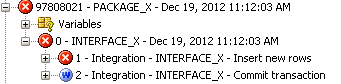
The interesting here is what he does behind the scenes. In the no-surrogate version ODI created one mapping for each hierarchy and in the end it merged everything together inside a table.

no-surrogate-time-operatorFor the Surrogate key version, ODI also generates one mapping for each hierarchy but the main difference is that after each one he merges it witch the others. This happens because he needs to get the surrogate key for each level.

time-surrogate-operator

For each level ODI automatically generates an insert into that level stage table verifying if all the columns does not exists in the target table (He does that to decrease the amount of data for the merge step since merge would insert or update everything and would take more time than necessary).

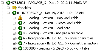
After the stage table is loaded the next step is to merge the stage table to the target table, and for that ODI just create a “Merge”: when match he updates the descriptions or attributes and when doesn’t match it inserts the new rows with the sequences for the SK.

In the next level of the hierarchy ODI repeats the process but joining the Year with the Quarter. ODI will keep doing this for each level mapped until the last one, where instead of having a merge with matches and not matches, he just do a merge with Matches (since he know everything will already be there).

The results will be this:

time-surrogate-table-results

It’s nice that ODI already creates the dimension thinking in an aggregated fact since we can see that he has some rows just with the year, other with the year and quarters and the last one with all the information.

One thing to notice is that the PK is the same as the Month SK. This is because ODI is ready to create SCD type 2 (we’ll do another post to show how it works).

For the fact, the mapping will still be the same as the No-surrogate version and again the difference will be in the results.

fact-surrogate-interface

We can see that in the operator ODI does something really neat this time.

fact-surrogate-operator

MERGE INTO EPM_HPT_ODI_RUN.S_FACT FACT_SURROGATE1_FACT_SURROGATE USING
(SELECT TIME_SURROGATE_FACT_SURROGAT_1.MONTH_SK AS ID_TIME ,
PRODUCT_SURROGATE_FACT_SURRO_1.PRODUCT_SK AS ID_PRODUCTS ,
REGIONS_SURROGATE_FACT_SURRO_1.CITY_SK AS ID_REGIONS ,
SRC_ERP.SALES AS METRIC
FROM ((EPM_HPT_ODI_RUN.SRC_ERP SRC_ERP
LEFT OUTER JOIN
(SELECT TIME_SURROGATE_FACT_SURROGATE.ID_MONTH AS ID_MONTH ,
TIME_SURROGATE_FACT_SURROGATE.MONTH_SK AS MONTH_SK ,
TIME_SURROGATE_FACT_SURROGATE.TIME_PK AS TIME_PK
FROM EPM_HPT_ODI_RUN.S_TIME TIME_SURROGATE_FACT_SURROGATE
WHERE ((TIME_SURROGATE_FACT_SURROGATE.TIME_PK = TIME_SURROGATE_FACT_SURROGATE.MONTH_SK)
AND (TIME_SURROGATE_FACT_SURROGATE.MONTH_SK IS NOT NULL) )
) TIME_SURROGATE_FACT_SURROGAT_1
ON (SRC_ERP.ID_MONTH = TIME_SURROGATE_FACT_SURROGAT_1.ID_MONTH) )
LEFT OUTER JOIN
(SELECT PRODUCT_SURROGATE_FACT_SURROGA.ID_PRODUCT AS ID_PRODUCT ,
PRODUCT_SURROGATE_FACT_SURROGA.PRODUCT_SK AS PRODUCT_SK ,
PRODUCT_SURROGATE_FACT_SURROGA.PRODUCTS_PK AS PRODUCTS_PK
FROM EPM_HPT_ODI_RUN.S_PRODUCTS PRODUCT_SURROGATE_FACT_SURROGA
WHERE ((PRODUCT_SURROGATE_FACT_SURROGA.PRODUCTS_PK = PRODUCT_SURROGATE_FACT_SURROGA.PRODUCT_SK)
AND (PRODUCT_SURROGATE_FACT_SURROGA.PRODUCT_SK IS NOT NULL) )
) PRODUCT_SURROGATE_FACT_SURRO_1
ON (SRC_ERP.ID_PRODUCT = PRODUCT_SURROGATE_FACT_SURRO_1.ID_PRODUCT) )
LEFT OUTER JOIN
(SELECT REGIONS_SURROGATE_FACT_SURROGA.ID_CITY AS ID_CITY ,
REGIONS_SURROGATE_FACT_SURROGA.CITY_SK AS CITY_SK ,
REGIONS_SURROGATE_FACT_SURROGA.REGIONS_PK AS REGIONS_PK
FROM EPM_HPT_ODI_RUN.S_REGIONS REGIONS_SURROGATE_FACT_SURROGA
WHERE ((REGIONS_SURROGATE_FACT_SURROGA.REGIONS_PK = REGIONS_SURROGATE_FACT_SURROGA.CITY_SK)
AND (REGIONS_SURROGATE_FACT_SURROGA.CITY_SK IS NOT NULL) )
) REGIONS_SURROGATE_FACT_SURRO_1
ON (SRC_ERP.ID_CITY = REGIONS_SURROGATE_FACT_SURRO_1.ID_CITY)
) MERGE_SUBQUERY ON ( FACT_SURROGATE1_FACT_SURROGATE.ID_TIME = MERGE_SUBQUERY.ID_TIME AND FACT_SURROGATE1_FACT_SURROGATE.ID_PRODUCTS = MERGE_SUBQUERY.ID_PRODUCTS AND FACT_SURROGATE1_FACT_SURROGATE.ID_REGIONS = MERGE_SUBQUERY.ID_REGIONS )
WHEN NOT MATCHED THEN
INSERT
(
ID_TIME ,
ID_PRODUCTS ,
ID_REGIONS ,
METRIC
)
VALUES
(
MERGE_SUBQUERY.ID_TIME ,
MERGE_SUBQUERY.ID_PRODUCTS ,
MERGE_SUBQUERY.ID_REGIONS ,
MERGE_SUBQUERY.METRIC
)
WHEN MATCHED THEN
UPDATE SET METRIC = MERGE_SUBQUERY.METRIC

He automatically joins all our dimensions at level zero (since we have the dimensions in the higher levels for the aggregated fact) to get the surrogate key information and use it in the fact table. This is very nice because in large DWs we’ll have tons of dimensions, and map/join everything is very time consuming. The final results is this:

fact-surrgoate-sql-results

A perfect DW created using surrogate key, in other words, instead of having the dimensions PKs in the fact table we have the SKs (that ware generated by a sequence in the dimensions).

In resume, we think that if you going to create simple dimensions and simple facts (without surrogate key or SCD type 2) it’s still nice to use this new feature since it’s a nice way to document and standardize your DW, but if we measure by development time it’s not worthy since it’s very time consuming for simple DW.

Now, if you want to create a DW using surrogate keys or SCD type 2 we found this new feature extremely useful for both, documentation and standardizations and because is a lot faster than do manually.

Thanks and see you soon.

Remotely Ziping files with ODI

Posted in 11.1.1.9.0, ACE, Configuration, EPM, Essbase, ETL, Hacking, Hyperion Essbase, InfraStructure, ODI, ODI 10g, ODI 11g, ODI 12c, ODI Architecture, ODI Architecture, OS Command, Performance, Remotely, Tips and Tricks, Zip Files with tags , , , , , , , , , , , on April 5, 2016 by RZGiampaoli

Hi guys how are you? It has been a long time since last time I wrote something but it was for a good reason! We were working in our two Kscope sessions! Yes, this year we will have 2 sessions and I think they will be great!

Anyway, let us get to the point!

Today I want to talk about something that should be very simple to do it but in the end, it is a nightmare…. Zip a file in a remote server…

A little bit of context! I was working in a backup interface for one client and, because their cubes are very big, I was trying to improve the performance as much as I can.

Part of the backup was to copy the .ind and .pag files and the data extract files as well. For an app we are talking in 30 gb of .pag and 40 gb of data extract files.

Their ODI infrastructure is like this:

Infrastructure

Basically I need to extract/copy data from Essbase server to the disaster recovery server (DR Server). Nothing special here. The problem is, because the size of the files I wanted to Zip the files first and then send it to the DR server.

If you use the ODI tools to Zip the file, what it does is bring all the files to the ODI Agent server, zip everything and the send it back. I really do not want all this traffic in the network and all the time lost in this process (also, the agent server is a LOT less powerful then the Essbase server).

Regular odi tools zip process

Then I start to research how I could do that (and thank you my colleague and friend Luis Fernando Cairo that help me a lot doing a lot of tests on this)

First of all we have three main options here:

  1. Create a .bat file and run it remotely: I did not like it because I do not want a lot of .bats all over the places
  2. Use windows invoke command: I need a program in the server like 7 zip or so and I don’t have access to install freely and I do not want to install zip’s program all over the places too
  3. Use Psexec to execute a program in the server: Same as the previous one.

Ok, I figure out that in the end I’ll need to create/install something in the server… and I rate it. Well, let’s at least optimize the problem right!

Then I was thinking, what I have in common in all Hyperion servers? The answer is JAVA.

Then I thought, I can use the JAR command to zip a file:

jar cfM file.zip *.pag *.ind

Where:

c: Creates a new archive file named jarfile (if f is specified) or to standard output (if f and jarfile are omitted). Add to it the files and directories specified by inputfiles.

f: Specifies the file jarfile to be created (c), updated (u), extracted (x), indexed (i), or viewed (t). The -f option and filename jarfile are a pair — if present, they must both appear. Omitting f and jarfile accepts a “jar file” from standard input (for x and t) or sends the “jar file” to standard output (for c and u).

M: Do not create a manifest file entry (for c and u), or delete a manifest file entry if one exists (for u).

Humm, things start to looks better. Now I had to decide if I would use the Invoke command or Psexec.

I started trying the Invoke command, but after sometime I figure out that I can’t execute the jar command using invoke.

Then my last alternative was Psexec.

The good thing about it is that is a zip file that you need just to unzip in the agent server, set it in the Environment Variables (PATH) and you are good to go.

It works amazingly.

You can run anything remotely with this and it’s a centralized solution and non-invasive as well (what I liked).

You just need to:

psexec \\Server  -accepteula  -w “work dir” javapath\jar cfM file.zip *.pag *.ind

Where:

-w: Set the working directory of the process (relative to remote computer).

-accepteula: This flag suppresses the display of the license dialog.

There’s one catch, for some unknown reason, the ODI agent does not get the PATH correctly then you need to use the complete path where it was “Installed”. The ODI is like this:

OdiOSCommand “-OUT_FILE=Log_Path/Zip_App_Files-RUM-PNL.Log” “-ERR_FILE =Log_Path /Zip_App_Files-RUM-PNL.err”

D:\Oracle\PSTools\psexec \\server -accepteula -w \\arborpath\APP\RUM\PNL\ JAVA_PATH\jdk160_35\bin\jar cfM App_Files-RUM-PNL.zip *.pag *.ind

With this, we will have a process like this:

Remotly Zip Process

This should not be something that complicate but it is and believe me, I create a very fast process and the client is very happy.

I hope you guys enjoy it and see you soon.

Dynamic topology configuration in ODI without using contexts

Posted in EPM, ODI Architecture with tags , , , , on August 12, 2013 by Rodrigo Radtke de Souza

— EDITED on Aug 12, 2015 —

Great news! Oracle just released “Patch 21156142: Parametric connections in ODI 12c don’t work anymore” which enables this technic to be used in ODI 12.1.3! Thanks Marius for this great tip!!!!

— End EDIT —

— EDITED on Dec 09, 2020—

5 years later, I had to implement this in ODI 12c and I could really test what some of the comments complained below. It seems that all variables works, but the password variable. However, if you use a GLOBAL variable, it works just fine. So, if you are in ODI 12c, please only use GLOBAL variables for this, otherwise you will have an issue in the password variable. Thanks!

— End EDIT —

— EDITED on May 6, 2015 —

Unfortunately, this technic only works on ODI 11 version. ODI 12c does not support dynamic password settings. We will let you know if we figure out a workaround for it.

— End EDIT —

Hi all, how are you doing? I came across this interesting situation during a project some time ago. Imagine the following scenario: You have a transactional system that was implemented in several places around the word. The system and its tables are exactly the same, but they are distributed across different databases, with different user names, database schemas, passwords, etc. Your task is to load data from this system with all these different database regions into your data warehouse, unifying all this data into one single place. Since all the tables have the same structures, how can you accomplish that with ODI without creating a lot of duplicate interfaces?

Everybody that already worked with ODI will easily answer that it may be accomplished using different contexts and they are totally right as we can see below:

image1

In resume, you create one interface object loading a table from the source system into your data warehouse and each context that you have created will point to a different database. It is just a matter to run that interface for each context and that’s it. However, there are situations where we cannot create that many contexts in a real production environment. In my case I couldn’t create those contexts because production execution repository is used for several other projects where those new contexts would just not make any sense at all. In production, the users have just one context called “Production” and they run any ODI job using that context, independently of the project which that ODI scenario belongs to. We could explain and teach the users to use multiple contexts, but my experience as a developer taught me that we need to let things as simple as possible to the end users, because there will be a day (for sure) that someone will execute a job using a wrong context and a mess may be created.

So, how can we accomplish this task without duplicating one interface per database that you need to load? Here is the technique:

Create one physical data server for each database that you need to load plus a dynamic data server:

image2

ADB_AMERICAS, ADB_APJ, ADB_EMEA and ADB_ZZ are the different databases that you need to connect and load data from. Those data servers are created as you normally create any data server in ODI and they will contain their own information regarding connection, data and work schemas and so on. In ADB_DYNAMIC you will create as the following:

Data Server:
User: #ODI_PROJECT.CONN_USER
Password: #ODI_PROJECT.CONN_PASS
JDBC URL: #ODI_PROJECT.CONN_URL

Physical Schema:
Schema: #ODI_PROJECT.CONN_DATA_USER
Work Schema: #ODI_PROJECT.CONN_WORK_USER

image3

image4 image5

As you can see, we have added five ODI variables in the topology information. These variables will be used to receive all the dynamic information from the different databases that we need to load. Now create one logical for each physical schema that you have created and point them accordingly in your context. Notice that we are also creating a logical schema called ADB_DYNAMIC that is going to point to our dynamic physical schema.

image13

Now this is an important step. Your models in ODI need to be pointing to ADB_DYNAMIC logical schema to make this work, but if you did not develop your interfaces yet and you also need to reverse your models and so on, you will not be able to do it pointing to this dynamic topology, since it has just ODI variables and not actual values there. So you will need to point your ADB_DYNAMIC logical schema temporally to a “normal” physical schema, let’s say ADB_AMERICAS to develop your interfaces. If you do this way, you will be able to reverse your models using ADB_DYNAMIC logical schema and you will be able to test all your interfaces pointing to one “valid” database without any additional work. After you complete your entire development, just point ADB_DYNAMIC logical schema back to ADB_DYNAMIC physical schema and proceed to the following step.

Now comes the tricky part. In order to make this technique to work, you will need to have a “control/parent” scenario that will call any “interfaces/child” scenarios passing as parameters all the connection information for each different database that you need to load. Let’s see an example:

image6

This child scenario contains all interfaces that will load your DW and it is receiving as parameters all connection information that will be used in ADB_DYNAMIC data server/physical schema. Remember that at this point, all interfaces are pointing to a physical schema that has only ODI variables on it, not actual values, so if you try to execute this package alone, it will not work. Now it is just a matter to call this scenario multiple times, one for each database that you need to load. First create a parent scenario with a procedure that will call those child scenarios as below:

image7

This procedure will have two steps for each database that you need to load. The first step will get one specific database connection and the second step will call the child scenario passing that connection information. It will look like this:

image8

If we open the first step, we will have the following:

image9

This step is creating Java variables that will temporally hold the connection information. These API commands are getting the connection information from the Command on Source tab, so in that tab we will have the following:

image10

We don’t need any code here. We just need the Schema combo box pointing to the desired database, in this case ADB_AMERICAS. This will allow all Java variables to get ADB_AMERICAS information that will be used in the next step which is the following:image11

This step will call the child scenario passing as parameters all the connection information that is needed to be used in ADB_DYNAMIC connection. When this child scenario runs, all interfaces inside of it will use ADB_AMERICAS connection information and will load data from it dynamically. Cool isn’t it? You are going to do the same configuration for the other steps in this procedure and the only thing that is going to change is the logical schema that you need to point in the “Command on Source” table. So “Get ADB_APJ Connections” will get ADB_APJ connection information and so on.

If you notice, this example is calling the child scenarios using SYNC_MODE=2, which means that they will execute the data load in all different databases in parallel, so if your architecture allows such parallelism, you may gain a great performance boost using this technique as well. We also added a “Wait for child scenarios” step as the last step, so we may control when all of the child scenarios have completed or not:

image12

So here is the end of this post. I hope you all enjoy!

Optimization Context in ODI

Posted in ODI Architecture with tags , , , , , on December 19, 2012 by Rodrigo Radtke de Souza

Hi all. I’ve decided to take a little break in our Hyperion Planning series to talk a about a “confusing” (and underestimated) feature in ODI: Optimization Context.

Optimization Context

This is a very important feature but few people know how to use it correctly.  This setting is used in design time to make ODI aware of how it should build its code. Let’s take a look at the following example:

Data Servers

For some reason (budget constraint, laziness, etc) the sales database schema that you want to read is in the same data server then your DW schema that you want to load in development. In production the situation changes and you have two separated data server, one for each schema.

Let’s say that we have two logical schemas, one for Sales (LOGICAL_SALES) and another for DW (LOGICAL_DW). In Development we created the following Physical Topology:

Dev Servers

In Production we have this:

Prod Servers

I will not go through all the small steps to replicate this here, but we need to set up the Physical/Context/Logical information, create the data models and reverse the tables. When we build the interface, things start to get interesting. Let’s take a look at the interface using the “Development” context in Optimization Context:

Flow Tab

In the Flow tab we have only one IKM to select because in the Development context our source and target physical schemas reside in the same data server. ODI uses the Optimization context to figure out how it is going to build its flow tab. Let’s change the Optimization context to Production now:

Optimization Context

Flow Tab

Well, it changed. Now we have one LKM and one IKM. Again ODI checked the Optimization context to build its flow tab. As Production has two separate data servers, ODI added a LKM to be able to load from one server to the other. So the Optimization context is the key parameter to let ODI know how to build its code. And it can be very tricky.

Imagine that we change back to Development Optimization context. Now we have just one IKM in the flow tab. Let’s save it and generate a scenario with that interface. If we run it using the Development context it will work fine because both schemas are in the same data server. But what happens if we run it using the Production context?

Operator Code

Operator Code

It failed. If we check the steps, we have just one “Insert new rows” that tries to insert into DW schema using a select in the Sales schema:

Operator Code

As in Production the schemas are in separated data servers and ODI created its flow tab using the Development Optimization context this code will never work. If we change the Optimization context to Production, regenerate the scenario and run it again, it will create additional LKM steps and it will work fine:

Operator Code

It is worth mentioning that the opposite is also true. Imagine that in Development you have different data servers, but in Production you have only one data server. If you use Development Optimization context ODI will create its code with a LKM and it will add extra steps that would not be necessary in the Production environment. This wouldn’t give you any error, but these extra steps will be redundant and will result in less performance.

So this concludes our post. Prior to select your Optimization context, find out which is your topology in all environments. In this way you will be sure that ODI will create the correct code for all environments without any extra steps or errors.

See ya!