Archive for Architecture

ODI Hidden Gems – SNP tables: Query to get executed code example

Posted in ODI, ODI 12c, ODI Architecture with tags , , on February 26, 2020 by Rodrigo Radtke de Souza

Hi all, today’s gem is something extremely useful that I’ve being using in every single project that I work on. Today’s gem is about SNP tables, which are the database tables that are used by ODI to store its metadata. When we install ODI, the installer asks us where we want to create our Master and Work repositories. Each repository contains a set of tables with different kind of information. From Oracle documentation:

  • Master Repository: This is a data structure containing information on the topology of the company’s IT resources, on security and on version management of projects and data models. This repository is stored on a relational database accessible in client/server mode from the different Oracle Data Integrator modules.
  • Work Repository: This is a data structure containing information about data models, projects, and their use. This repository is stored on a relational database accessible in client/server mode from the different Oracle Data Integrator modules.

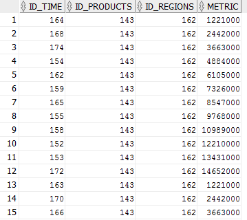
You may think of them being the place where contains all information about the code that was developed in ODI, all the jobs that were executed, all the source and target tables and so on. These tables may give us answers to questions like: how many mapping objects does project X have? Which are the target mappings for a specific job? How many jobs are executing in a daily basis, how long does each of them take and how much data do they manipulate (insert/delete/update)? All those questions will eventually come to you after some time, and querying the SNP tables will provide you all the answers on what is going on in your ODI projects.

Below is one example of a query that returns a lot of information regarding all the ODI executions that happened in an ODI repository in a give time frame. It gives you the name of the scenarios, versions, when it began and ended, the session status, the order that they happened and (maybe the most important) which code was executed. The last info, together with how much time it took to execute, may be very useful to analyze which are the steps that are taking longer in your environment and then do something about them.

I wont go over each table and what they mean, but you may take a look on “Doc ID 1903225.1 : Oracle Data Integrator 11g and 12c Repository Description” in Oracle support for a full list of tables and their description. In the beginning, the number of tables and attributes may look intimidating, but once you start to use them you will see that the data architechture is fairly simple and you may retrieve a lot of good information out of them.

Without further due, here is the SQL. This one was created over ODI 12.2.1. Please notice that each ODI version may have changes in the repositories tables, which may lead you to modify those queries accordingly.

SELECT
SS.SESS_NO,
SS.SCEN_NAME,
SS.SCEN_VERSION,
SS.SESS_NAME,
SS.PARENT_SESS_NO,
SS.SESS_BEG,
SS.SESS_END,
SS.SESS_STATUS,
DECODE(SS.SESS_STATUS,'D','Done','E','Error','M','Warning','Q','Queued','R','Running','W','Waiting',SS.SESS_STATUS) AS SESS_STATUS_DESC,
SSL.NNO,
SSTL.NB_RUN,
SST.TASK_TYPE,
DECODE(SST.TASK_TYPE,'C','Loading','J','Mapping','S','Procedure','V','Variable',SST.TASK_TYPE) AS TASK_TYPE_DESC,
SST.EXE_CHANNEL,
DECODE(SST.EXE_CHANNEL,'B','Oracle Data Integrator Scripting','C','Oracle Data Integrator Connector','J','JDBC','O','Operating System'
,'Q','Queue','S','Oracle Data Integrator Command','T','Topic','U','XML Topic',SST.EXE_CHANNEL) AS EXE_CHANNEL_DESC,
SSTL.SCEN_TASK_NO,
SST.PAR_SCEN_TASK_NO,
SST.TASK_NAME1,
SST.TASK_NAME2,
SST.TASK_NAME3,
SSTL.TASK_DUR,
SSTL.NB_ROW,
SSTL.NB_INS,
SSTL.NB_UPD,
SSTL.NB_DEL,
SSTL.NB_ERR,
SSS.LSCHEMA_NAME
|| '.'
|| SSS.RES_NAME AS TARGET_TABLE,
CASE
WHEN SST.COL_TECH_INT_NAME IS NOT NULL
AND SST.COL_LSCHEMA_NAME IS NOT NULL THEN SST.COL_TECH_INT_NAME
|| '.'
|| SST.COL_LSCHEMA_NAME
ELSE NULL
END AS TARGET_SCHEMA,
SSTL.DEF_TXT AS TARGET_COMMAND,
CASE
WHEN SST.DEF_TECH_INT_NAME IS NOT NULL
AND SST.DEF_LSCHEMA_NAME IS NOT NULL THEN SST.DEF_TECH_INT_NAME
|| '.'
|| SST.DEF_LSCHEMA_NAME
ELSE NULL
END AS SOURCE_SCHEMA,
SSTL.COL_TXT AS SOURCE_COMMAND
FROM
SNP_SESSION SS
INNER JOIN SNP_STEP_LOG SSL ON SS.SESS_NO = SSL.SESS_NO
INNER JOIN SNP_SESS_TASK_LOG SSTL ON SS.SESS_NO = SSTL.SESS_NO
INNER JOIN SNP_SB_TASK SST ON SSTL.SB_NO = SST.SB_NO
AND SSTL.SCEN_TASK_NO = SST.SCEN_TASK_NO
AND SSL.NNO = SSTL.NNO
AND SSTL.NNO = SST.NNO
AND SSL.NB_RUN = SSTL.NB_RUN
LEFT JOIN SNP_SB_STEP SSS ON SST.SB_NO = SSS.SB_NO
AND SST.NNO = SSS.NNO
WHERE
SS.SESS_BEG >= TRUNC(SYSDATE) - 1
ORDER BY
SESS_NO,
NNO,
SCEN_TASK_NO

See ya!

ODI 12c new features: Dimension and Cubes! Part 4 (Loading using Surrogate Keys)

Posted in Dimensions, ETL, ODI 12c, ODI Architecture, ODI Mapping, Oracle, Tips and Tricks with tags , , , , , on December 16, 2016 by RZGiampaoli

Hi guys how are you?

Today we’ll continue the dimension and cubes series (Part 1, Part2 and Part 3 here) and we’ll see how to load data using Surrogate keys.

After all the setting done in the last post, now the only thing left is to create the interfaces and map everything. For the Surrogate keys, the interface and the mapping are exactly the same as for no-surrogate version (as we can see in the previous posts) for both, dimensions and facts, what’s very nice.

times-surrogate-interfaceThe interesting here is what he does behind the scenes. In the no-surrogate version ODI created one mapping for each hierarchy and in the end it merged everything together inside a table.

no-surrogate-time-operatorFor the Surrogate key version, ODI also generates one mapping for each hierarchy but the main difference is that after each one he merges it witch the others. This happens because he needs to get the surrogate key for each level.

time-surrogate-operator

For each level ODI automatically generates an insert into that level stage table verifying if all the columns does not exists in the target table (He does that to decrease the amount of data for the merge step since merge would insert or update everything and would take more time than necessary).

After the stage table is loaded the next step is to merge the stage table to the target table, and for that ODI just create a “Merge”: when match he updates the descriptions or attributes and when doesn’t match it inserts the new rows with the sequences for the SK.

In the next level of the hierarchy ODI repeats the process but joining the Year with the Quarter. ODI will keep doing this for each level mapped until the last one, where instead of having a merge with matches and not matches, he just do a merge with Matches (since he know everything will already be there).

The results will be this:

time-surrogate-table-results

It’s nice that ODI already creates the dimension thinking in an aggregated fact since we can see that he has some rows just with the year, other with the year and quarters and the last one with all the information.

One thing to notice is that the PK is the same as the Month SK. This is because ODI is ready to create SCD type 2 (we’ll do another post to show how it works).

For the fact, the mapping will still be the same as the No-surrogate version and again the difference will be in the results.

fact-surrogate-interface

We can see that in the operator ODI does something really neat this time.

fact-surrogate-operator

MERGE INTO EPM_HPT_ODI_RUN.S_FACT FACT_SURROGATE1_FACT_SURROGATE USING
(SELECT TIME_SURROGATE_FACT_SURROGAT_1.MONTH_SK AS ID_TIME ,
PRODUCT_SURROGATE_FACT_SURRO_1.PRODUCT_SK AS ID_PRODUCTS ,
REGIONS_SURROGATE_FACT_SURRO_1.CITY_SK AS ID_REGIONS ,
SRC_ERP.SALES AS METRIC
FROM ((EPM_HPT_ODI_RUN.SRC_ERP SRC_ERP
LEFT OUTER JOIN
(SELECT TIME_SURROGATE_FACT_SURROGATE.ID_MONTH AS ID_MONTH ,
TIME_SURROGATE_FACT_SURROGATE.MONTH_SK AS MONTH_SK ,
TIME_SURROGATE_FACT_SURROGATE.TIME_PK AS TIME_PK
FROM EPM_HPT_ODI_RUN.S_TIME TIME_SURROGATE_FACT_SURROGATE
WHERE ((TIME_SURROGATE_FACT_SURROGATE.TIME_PK = TIME_SURROGATE_FACT_SURROGATE.MONTH_SK)
AND (TIME_SURROGATE_FACT_SURROGATE.MONTH_SK IS NOT NULL) )
) TIME_SURROGATE_FACT_SURROGAT_1
ON (SRC_ERP.ID_MONTH = TIME_SURROGATE_FACT_SURROGAT_1.ID_MONTH) )
LEFT OUTER JOIN
(SELECT PRODUCT_SURROGATE_FACT_SURROGA.ID_PRODUCT AS ID_PRODUCT ,
PRODUCT_SURROGATE_FACT_SURROGA.PRODUCT_SK AS PRODUCT_SK ,
PRODUCT_SURROGATE_FACT_SURROGA.PRODUCTS_PK AS PRODUCTS_PK
FROM EPM_HPT_ODI_RUN.S_PRODUCTS PRODUCT_SURROGATE_FACT_SURROGA
WHERE ((PRODUCT_SURROGATE_FACT_SURROGA.PRODUCTS_PK = PRODUCT_SURROGATE_FACT_SURROGA.PRODUCT_SK)
AND (PRODUCT_SURROGATE_FACT_SURROGA.PRODUCT_SK IS NOT NULL) )
) PRODUCT_SURROGATE_FACT_SURRO_1
ON (SRC_ERP.ID_PRODUCT = PRODUCT_SURROGATE_FACT_SURRO_1.ID_PRODUCT) )
LEFT OUTER JOIN
(SELECT REGIONS_SURROGATE_FACT_SURROGA.ID_CITY AS ID_CITY ,
REGIONS_SURROGATE_FACT_SURROGA.CITY_SK AS CITY_SK ,
REGIONS_SURROGATE_FACT_SURROGA.REGIONS_PK AS REGIONS_PK
FROM EPM_HPT_ODI_RUN.S_REGIONS REGIONS_SURROGATE_FACT_SURROGA
WHERE ((REGIONS_SURROGATE_FACT_SURROGA.REGIONS_PK = REGIONS_SURROGATE_FACT_SURROGA.CITY_SK)
AND (REGIONS_SURROGATE_FACT_SURROGA.CITY_SK IS NOT NULL) )
) REGIONS_SURROGATE_FACT_SURRO_1
ON (SRC_ERP.ID_CITY = REGIONS_SURROGATE_FACT_SURRO_1.ID_CITY)
) MERGE_SUBQUERY ON ( FACT_SURROGATE1_FACT_SURROGATE.ID_TIME = MERGE_SUBQUERY.ID_TIME AND FACT_SURROGATE1_FACT_SURROGATE.ID_PRODUCTS = MERGE_SUBQUERY.ID_PRODUCTS AND FACT_SURROGATE1_FACT_SURROGATE.ID_REGIONS = MERGE_SUBQUERY.ID_REGIONS )
WHEN NOT MATCHED THEN
INSERT
(
ID_TIME ,
ID_PRODUCTS ,
ID_REGIONS ,
METRIC
)
VALUES
(
MERGE_SUBQUERY.ID_TIME ,
MERGE_SUBQUERY.ID_PRODUCTS ,
MERGE_SUBQUERY.ID_REGIONS ,
MERGE_SUBQUERY.METRIC
)
WHEN MATCHED THEN
UPDATE SET METRIC = MERGE_SUBQUERY.METRIC

He automatically joins all our dimensions at level zero (since we have the dimensions in the higher levels for the aggregated fact) to get the surrogate key information and use it in the fact table. This is very nice because in large DWs we’ll have tons of dimensions, and map/join everything is very time consuming. The final results is this:

fact-surrgoate-sql-results

A perfect DW created using surrogate key, in other words, instead of having the dimensions PKs in the fact table we have the SKs (that ware generated by a sequence in the dimensions).

In resume, we think that if you going to create simple dimensions and simple facts (without surrogate key or SCD type 2) it’s still nice to use this new feature since it’s a nice way to document and standardize your DW, but if we measure by development time it’s not worthy since it’s very time consuming for simple DW.

Now, if you want to create a DW using surrogate keys or SCD type 2 we found this new feature extremely useful for both, documentation and standardizations and because is a lot faster than do manually.

Thanks and see you soon.

ODI 12c new features: Dimension and Cubes! Part 2 (Loading using Natural Keys)

Posted in Cubes, Dimensions, ETL, New Features, ODI 12c, ODI Architecture with tags , , , , , on September 14, 2016 by Rodrigo Radtke de Souza

Hi all, let’s continue with our posts regarding “ODI 12c new features: Dimension and Cubes”. As stated in the previous post, we can have two ways to build our new objects: with natural keys or with surrogate keys. Today’s post will focus on loading the dimensions and fact tables that where created using natural keys (please see our previous post for all the settings required for those objects).

Let’s begin loading our TIME dimension (which was mapped to our TIME Oracle table). This dimension will have information from three different source tables: SRC_YEAR, SRC_QUARTER and SRC_MONTH. Each of them has information regarding each TIME hierarchy level, so all of them needs to be loaded in order to have a complete hierarchy in our final table.

The load process is very easy and intuitive: first create a new mapping and drag and drop the TIME dimension to it. Then, just add the three source tables, map to its correspondent level in the TIME dimension and that’s it. A very cool thing here is that ODI understands each level as a “separate” table/process, so you don’t need to join your source tables before actually loading it to the target dimension. In other words, ODI allows you to have any kind of complex ETL to each dimension level and each level will be treated as “separate” data loads that will be glued together by the hierarchy setting that you mapped in the TIME dimension object. Here is what it looks like:

blog1

blog2

blog3

blog4

When you execute the mapping we are going to see that the first “MAP_BEGIN” section will try to create and truncate our stage tables that were set in our dimension object. Here is an odd thing (as we also mentioned in the last post): We could not understand yet why ODI “forces” you to have the stage tables created prior to execution (so you can select them in the Dimension object), as it could very well create them for you (like it does for C$ and I$ tables). I know that Oracle may had a reason behind it, but as for now, the entire “stage tables” thing seems an unnecessary setup. Anyway, the important thing here is that ODI will truncate the stage tables before any new execution.

blog5

In the “MAP_MAIN” section is where it gets interesting. We can see here how ODI threats this new dimension object: each level has its own ETL, as we can see that it is loading YEAR, QUARTER and MONTH separately. First YEAR step will load its source to its stage table STG_YEAR, then QUARTER step will join the information from its source table plus STG_YEAR to its STG_QUARTER table. Finally, MONTH step, that is our leaf/grain level, will join its source table plus STG_QUARTER table (which is already joined with YEAR source) and merge it all together in our final table TIME. The result will look like below:

blog6

Since we are not using Surrogate keys here, our Dimension table will contain only the grain/leaf members with all Natural Keys and its attributes for all levels that exists in the dimension. So one row will contain all information regarding all levels that it belongs to. When we create the mappings for the other two dimensions (they’re very similar, so I’m not adding them here) and execute them, we will get the following results:

blog7

blog8

Let’s to go our Fact table load. This one is way too simple, since our source table already contains all the Natural Keys that will be the ones that will also exist in our FACT table (remember, we are not dealing with Surrogate Keys in this example). Here we just need to map each NK to its respective dimension column and also our Measure data and execute the mapping.

blog9

blog10

When we take a look in Operator, we are going to see a single merge command in our Fact table, where ODI will use all dimensions to search if that row already exists in our FACT table. If it exists, the measure column is update, otherwise it is inserted.

blog11

The final result is below: as expected, all Natural Keys from our dimensions were inserted in the Fact table, together with our measure.

blog12

Now you may be wondering, why should I use these new features if it seems a lot of work (settings) for a little gain? Well, using ODI for Natural Key’s only is really not worth it, since the only benefit here seems to be ODI loading the dimensions levels all at once, with different sources/ETL, in a single mapping object, which is a very cool feature, since it enables us to better organize our DW objects and have a clear view on our ETL logic. But again, this is too little for the amount of work that we need to do to get there. But don’t worry, it will get way better when we start to work with Surrogate Keys, since ODI will be able to abstract all the Surrogate Key management and you will start to feel that all the necessary settings will finally be worth the work.

That’s it for today folks! We will be releasing the Surrogate Key settings and load posts very soon, so stay tuned in our blog! See ya!

ODI 12c new features: Dimension and Cubes! Part 1 (Settings)…

Posted in ACE, Configuration, Cubes, Dimensions, ETL, New Features, ODI, ODI 12c, ODI Architecture, ODI Mapping, Tips and Tricks with tags , , , , , , , , on August 19, 2016 by RZGiampaoli

Today we’ll talk a little bit about the new feature introduced in ODI 12.2.1.1.0, Dimension and Cubes!

As everybody already know, Oracle is slowly merging OWB within ODI and in each release we can see a new feature from OWB arriving in ODI. This time were the Dimension and Cubes feature.

This feature helps you to create a DW based in a configuration that you do. Basically there is a new component in ODI that helps you to define the datastore to be mapped. Also, after you create all dimensions (that is the most time consuming part in the process), the cube or fact table creation and mapping is a lot easier than do it manually.

Right now there is just one type of dimension available (Star schema level based dimension), but in the future other kinds will be supported like snow flake and others.

Ok, let’s start. There’re two ways to build a star dimension in ODI: with natural key’s (where the natural key is stored in the FACT table) and with surrogate keys (where the surrogate key is stored in the FACT table). In this post we’ll cover how we create a DW using the natural key process since the surrogate key one is buggy (the interface fails on saving the surrogate key) and we have openned a SR with Oracle to get it fixed. As soon we have the fix we’ll cover that too here in the blog.

In the Designer tab we can now see that we have a new tab called Dimensions and Cubes.

1-Dimension and Cubes

Opening that tab you will find a blank area, you need to click the button in the “Dimension and Cubes” tab, and you can create a new DM or DW.

2-DW creation

By the way, here’s the first small bug. For some reason when you write the name you want, ODI does not fill automatically the code field (as it always do for all the other objects in ODI), then you need to manually insert a code there. Remember, no spaces and no special character.

After that we can expand it and see the Dimension and the Cube node.

3-DW creation

Right click on those and we can create a new Dimension or Cube. As everybody knows, the dimension comes first since we need them to maintain the data integrity of the cube.

4-Dimension Definition

Here you can give any name you want for the dimension. Also you have a Pattern Name (that has just one option by now) and in the side tabs we have all possible options for the Dimension, Levels and Hierarchies, that we’ll cover later.

There are two more option here: the Datastore, that is the target dimension datastore where all metadata will flow and the Surrogate key Sequence that you need to set in case you want to create a dim using surrogate key (We’ll cover this later since we have a bug here).

In our case we’ll have three dimensions and one cube. (Time, Products, Regions and Fact). Both the source and the targets tables were generated by me with dummy data, just for this post. If you want to replicate this example, the scripts are here:

No surrogate Script

Let’s create the Time dimension. Click in the “Levels” in the left side tabs and you will see a big screen in three big sessions: Levels, Levels Attributes and Parent Level References.

5-Level Canvas

Let’s begin with the level configuration. Clicking in the Plus Sign button will create a Level.

6-Level Creation

I always like to rename the Level to something more meaningful like “Year” but if you like you can keep as default. By the default the target datastore comes automatically mapped since you define it in the previous screen. The only thing left here is to define the “Staging Datasore”.

This is something that we didn’t understood why it was made in this way since ODI could create automatically based in the definitions we had in the previous step or even with the interface configuration.

Anyway, what we need to do is create the stage tables for each level, and for that we have a few approaches we can do here:

  1. We can create another table exactly in the same way of the target table (needs to be a new table because the way ODI integrates the data. We’ll cover that latter).
  2. We can create, in this case, 3 tables, one for Year (same way as the source table is), and one for Quarter (same way of the source plus all columns from the Year table) and one for Month (same way of the source plus Quarter and Year columns).
  3. And we can duplicate the sources or the target datastore and do the changes above (in the 2 approach).

With the Stage datastores created (manually or by reverse) we just need to click in the “…” button and choose it from the list. Now we just need to repeat the step 2 more times for the other levels:

7-Level Canvas mapps

After we associate the source datastores and the stage datastores it’s time to create the attributes and ID’s for each level. For this you just need to click in the Year level and click in the Plus Sign button below:

8-Level attibutes config

Here we need to create all the attributes for this level and the natural key for that level as well. (We have the option to create slowly change dimensions here, but this will be covered in a future post!)

For each attribute you need to Plus Sign and fill the name of the attribute, set the data type (yes it not get automatically….) and select the Stage attribute (click in the “…” button and select it).

After all Attributes and ID’s we need to click in the below Plus Sign to set the natural key of that level. Just select in the list available.

After that, we just need to repeat for all the other 2 levels that we’ll have in this dimension.

With this done, the last step for this tab is to create the relationship between one level and its parent level. For this, highlight each level again, in this case we’ll start from bottom up, then let’s start clicking in the Month level and click on Plus Sign button below. Here we just need to say that for the Month level his reference parent will be Quarter. To set this we just need to select the Quarter level from the drop box and select eh foreign key from the drop box as well. Do that again for the Quarter level and reference it to the Year level. We don’t need to create any reference for the Year since it has no parent.

9 Parent Level References

As you can see, after the level configuration, everything you need to do is click in buttons and select from drop box or from “…” Screen (other than rename the defaults values if you like).
For last but not least, we need to click in the tab Hierarchies on the left tabs to enable us create a new hierarchy.

This is something fun. We can create multiple hierarchies inside the target table as well as skip level and some other features that we’ll cover in another post. For now let’s stay with a single hierarchy.

10-hierarchy

Here we need just to create the hierarchy by clicking in the Plus Sign button, give a name for the hierarchy and then click in the plus button bellow and add all the levels for the hierarchy. The order doesn’t matter, the idea here is that you can have multiple hierarchies with different levels in each one. For example, we could have a hierarchy called Full_Time with Year->Quarter->Month and another Hierarchy called Small_Time with just Year->Month. ODI would know based in the configurations we did, how to handle the data. Nice.

Also we can set skip level for each level we defined.

We are done with the dimension settings. I know it’s a lot of settings and some of you could be thinking (as we thought, this is a lot more work than if I create manually), but believe me, after you get used, you can do it in a reasonable time and the cube part is worthy.

Now we just need to repeat the process for all the other 2 dimension and them we finally start the cube settings:

11-Cube

To start the same thing as the dimension, Right click in the Cubes node and new.

12-Cube definition

In this screen we need to give a name for the cube, select a pattern name (Same as Dimension, just one option here for now) and do a biding to the target datastore.
After that we just need to click in the Detail tab in the left menu and start to configure our fact table.

12-Cube config

As I said in the beginning, here’s where the use of this components pays off. To configure a cube we just need click in the Plus Sign button and add all dimension we have, in this case our three dimensions. Then we just need to select the level we want to join our Fact table with our dimensions and bind the keys from the fact and that dimension.

For the last but not the least we just need to create by Plus Sign the measures that the Fact table will have. Same as the attributes in the dimensions: Name of the measure, Datatype and the column that will receive the data.

And that’s it. We are all set to move to the Mappings. Since this is already a huge post, I’ll stop this one now and will start a new post just for the Mappings, since I want to analyze how ODI builds the queries and loads the data there.

Hope you guys enjoy this post and see you soon.

Let’s Join DEVEPM @ KSCOPE 16

Posted in ACE, EPM, Essbase, ETL, Hyperion Essbase, Hyperion Planning, InfraStructure, Kscope 16, ODI, ODI 10g, ODI 11g, ODI 12c, ODI Architecture, ODTUG, Oracle Database, OS Command, Performance, Tips and Tricks with tags , , , , , , , , , , , , on April 5, 2016 by RZGiampaoli

Hi Guys how are you?

Just a quickly post about this year KSCOPE. This year we’ll have 2 excellent sessions:

Take a Peek at Dell’s Smart EPM Global Environment:

Ricardo Giampaoli , TeraCorp

Co-presenter(s): Rodrigo Radtke de Souza, Dell

When: Jun 27, 2016, Session 2, 10:15 am – 11:15 am

Topic: EPM Applications – Subtopic: Planning

In a fast-moving business environment, finance leaders are successfully leveraging technology advancements to transform their finance organizations and generate value for the business.
Oracle’s Enterprise Performance Management (EPM) applications are an integrated, modular suite that supports a broad range of strategic and financial performance management tools that help business to unlock their potential.

Dell’s global financial environment contains over 10,000 users around the world and relies on a range of EPM tools such as Hyperion Planning, Essbase, Smart View, DRM, and ODI to meet its needs.

This session shows the complexity of this environment, describing all relationships between those tools, the techniques used to maintain such a large environment in sync, and meeting the most varied needs from the different business and laws around the world to create a complete and powerful business decision engine that takes Dell to the next level. 

Incredible ODI Tips to Work with Hyperion Tools

Ricardo Giampaoli , TeraCorp

Co-presenter(s): Rodrigo Radtke de Souza, Dell

When: Jun 27, 2016, Session 6, 4:30 pm – 5:30 pm

Topic: EPM Platform – Subtopic: EPM Data Integration

ODI is an incredible and flexible development tool that goes beyond simple data integration. But most of its development power comes from outside-the-box ideas.

  • Did you ever want to dynamically run any number of “OS” commands using a single ODI component?
  • Did you ever want to have only one data store and loop different sources without the need of different ODI contexts?
  • Did you ever want to have only one interface and loop any number of ODI objects with a lot of control?
  • Did you ever need to have a “third command tab” in your procedures or KMs to improve ODI powers?
  • Do you still use an old version of ODI and miss a way to know the values of the variables in a scenario execution?
  • Did you know ODI has four “substitution tags”? And do you know how useful they are?
  • Do you use “dynamic variables” and know how powerful they can be?
  • Do you know how to have control over you ODI priority jobs automatically (stop, start, and restart scenarios)?

If you want to know the answer to all this questions, please join us in this session to learn the special secrets of ODI that will take your development skills to the next level.

Join us in KSCOPE 16 and book our 2 sessions in schedule. They will be very good sessions and I’m sure that you’ll learn some new stuff that will help you in your EPM Environment!

SpeakerSquare (1)

Remotely Ziping files with ODI

Posted in 11.1.1.9.0, ACE, Configuration, EPM, Essbase, ETL, Hacking, Hyperion Essbase, InfraStructure, ODI, ODI 10g, ODI 11g, ODI 12c, ODI Architecture, ODI Architecture, OS Command, Performance, Remotely, Tips and Tricks, Zip Files with tags , , , , , , , , , , , on April 5, 2016 by RZGiampaoli

Hi guys how are you? It has been a long time since last time I wrote something but it was for a good reason! We were working in our two Kscope sessions! Yes, this year we will have 2 sessions and I think they will be great!

Anyway, let us get to the point!

Today I want to talk about something that should be very simple to do it but in the end, it is a nightmare…. Zip a file in a remote server…

A little bit of context! I was working in a backup interface for one client and, because their cubes are very big, I was trying to improve the performance as much as I can.

Part of the backup was to copy the .ind and .pag files and the data extract files as well. For an app we are talking in 30 gb of .pag and 40 gb of data extract files.

Their ODI infrastructure is like this:

Infrastructure

Basically I need to extract/copy data from Essbase server to the disaster recovery server (DR Server). Nothing special here. The problem is, because the size of the files I wanted to Zip the files first and then send it to the DR server.

If you use the ODI tools to Zip the file, what it does is bring all the files to the ODI Agent server, zip everything and the send it back. I really do not want all this traffic in the network and all the time lost in this process (also, the agent server is a LOT less powerful then the Essbase server).

Regular odi tools zip process

Then I start to research how I could do that (and thank you my colleague and friend Luis Fernando Cairo that help me a lot doing a lot of tests on this)

First of all we have three main options here:

  1. Create a .bat file and run it remotely: I did not like it because I do not want a lot of .bats all over the places
  2. Use windows invoke command: I need a program in the server like 7 zip or so and I don’t have access to install freely and I do not want to install zip’s program all over the places too
  3. Use Psexec to execute a program in the server: Same as the previous one.

Ok, I figure out that in the end I’ll need to create/install something in the server… and I rate it. Well, let’s at least optimize the problem right!

Then I was thinking, what I have in common in all Hyperion servers? The answer is JAVA.

Then I thought, I can use the JAR command to zip a file:

jar cfM file.zip *.pag *.ind

Where:

c: Creates a new archive file named jarfile (if f is specified) or to standard output (if f and jarfile are omitted). Add to it the files and directories specified by inputfiles.

f: Specifies the file jarfile to be created (c), updated (u), extracted (x), indexed (i), or viewed (t). The -f option and filename jarfile are a pair — if present, they must both appear. Omitting f and jarfile accepts a “jar file” from standard input (for x and t) or sends the “jar file” to standard output (for c and u).

M: Do not create a manifest file entry (for c and u), or delete a manifest file entry if one exists (for u).

Humm, things start to looks better. Now I had to decide if I would use the Invoke command or Psexec.

I started trying the Invoke command, but after sometime I figure out that I can’t execute the jar command using invoke.

Then my last alternative was Psexec.

The good thing about it is that is a zip file that you need just to unzip in the agent server, set it in the Environment Variables (PATH) and you are good to go.

It works amazingly.

You can run anything remotely with this and it’s a centralized solution and non-invasive as well (what I liked).

You just need to:

psexec \\Server  -accepteula  -w “work dir” javapath\jar cfM file.zip *.pag *.ind

Where:

-w: Set the working directory of the process (relative to remote computer).

-accepteula: This flag suppresses the display of the license dialog.

There’s one catch, for some unknown reason, the ODI agent does not get the PATH correctly then you need to use the complete path where it was “Installed”. The ODI is like this:

OdiOSCommand “-OUT_FILE=Log_Path/Zip_App_Files-RUM-PNL.Log” “-ERR_FILE =Log_Path /Zip_App_Files-RUM-PNL.err”

D:\Oracle\PSTools\psexec \\server -accepteula -w \\arborpath\APP\RUM\PNL\ JAVA_PATH\jdk160_35\bin\jar cfM App_Files-RUM-PNL.zip *.pag *.ind

With this, we will have a process like this:

Remotly Zip Process

This should not be something that complicate but it is and believe me, I create a very fast process and the client is very happy.

I hope you guys enjoy it and see you soon.

Reviewing “Developing Essbase Applications – Hybrid Techniques and Practices” from an ETL Architect perspective

Posted in Book, EPM, Review with tags , , , , , on January 8, 2016 by Rodrigo Radtke de Souza

Hi guys! Today we are very happy to be reviewing “Developing Essbase Applications – Hybrid Techniques and Practices” for you. We will review the book not once, but twice and the reason behind that is that Ricardo and I (Rodrigo) have different backgrounds and this creates very different opinions around the book topics.

My professional career comes much more strongly from an ETL Architect position, so although I know the basics and principals around Essbase, for me it was always one more target/source system to pull/retrieve data from. Ricardo in the other hand has his major years working with EPM space and he knows/uses Essbase at its fullest. So based on that, let’s see how our reviews will differ from one another!

51QGgxNE-vL._SX340_BO1,204,203,200_

ETL Architect perspective review

Developing Essbase Applications – Hybrid Techniques and Practices” may be considered the “second” book of the “Developing Essbase Application” series (“Developing Essbase Applications: Advanced Techniques for Finance and IT Professionals” is the first one and it is a must to have!) but it is completely different from the first book, since it cover different topics with some different authors. Speaking on topics, this is what you will find in “Hybrid Techniques and Practices”:

  • Exalytics
  • Hybrid Essbase
  • Young Person’s Guide to Essbase Cube Design
  • Essbase Performance and Load Testing
  • Utilizing SQL to Enhance Essbase
  • Integrating OBIEE and Essbase
  • Managing Spreadsheets with Dodeca
  • Smart View

The books is edited by Cameron Lackpour along with John Booth, Tim German, William Hodges, Mike Nader, Martin Neuliep, and Glenn Schwartzberg. Those names are more than a reference in the EPM community and it is great to see great minds putting their effort to create this book. We know that anything in life (it can be a book/work/presentation/project) will be great when the people that are involved in that process are passionate about what they do and this is well represented here. All these people just love EPM/Essbase and this passion alongside with their great knowledge about the topics created a fantastic book.

The chapters in the book are well separated, so you may read any topic in any order that you prefer. First topic will talk about Exalytics and its “Secret Sauce”. Hardware aficionados will love this chapter, but “not-hardware guys” like me may fell kind of lost. I got that Exalytics is great and do great things for Essbase, but all metrics and hardware comparison tables I’ll just leave for the hardware/environment guys 🙂

The second chapter for me is the shiny gem of the book and it alone is already worth the cost of the book (it couldn’t be different, since this chapter is also the book’s title). Hybrid is a very new concept in the Essbase world so you will read what it is, its architecture, what you can/can’t do with Hybrid right now and so on. For someone to understand what Hybrid means, he must also understand the concepts of ASO/BSO and these are well covered in this chapter as well. In resume, this is fantastic overview what Hybrid currently is and how to get along with it.

I read the third chapter before I got the book because it is available for free on OTN!  You may download it and read it entirely! This chapter I would recommend to everyone that will have any kind of iteration with Essbase, especially those people that ask requirements to be implemented :). Although the information may be considered “basic” Essbase design, it is the core foundation to have a good Essbase implementation. Fantastic chapter and as I said, it is free, so go there and read it (after you finish to read the rest of the post, of course)!

I was extremely glad to read chapter 4 because it talks about Essbase performance and load test. This kind of subject is very rare to be found and this chapter contains a very good overview on some techniques that could be applied to have a performance test on Essbase. This is a complicated topic since testing Essbase is not a trivial thing. There are too many factors to consider but this chapter does a great job explaining those details and how you could accomplish a good test scenario.

On the very beginning of chapter five, Glenn states that his chapter contains very basic information about SQL and if you know SQL already you may just skip the first part of it. Since SQL is in my blood for some years now, I skipped almost the entire chapter, just reading the end of it when it talks about how to use SQL within Essbase. This chapter is for people that uses Essbase but are now aware of what SQL could do for them. My opinion is that everyone that “works with numbers” should know at the least the basic concepts of SQL and it heavily applies for Essbase users.

Chapter 6 will give you a very good perspective of what you can do when reporting Essbase using OBIEE, its limitations, its good practices and the workarounds that may be used to implement some of the most common requirements that are “not natively” supported by the tool. A great chapter that I’ll just keep coming back to it whenever I have some doubt about the do’s and don’ts around Essbase and OBIEE integration.

I’ll talk about chapter 7 and 8 together since they talk about tools that can be used to interact with Essbase data. I must say that I just use Smart view to check if something got loaded or to do some basic tie out checks, so my iteration with those tools are pretty basic. Chapter 7 talks all about Dodeca and I got some pretty interesting information that I was not aware of, like its architecture, how it differs from other tools and so on. Chapter 8 goes deep into Smart View and tell us how it can be customized to allow the users to retrieve more value from the tool. From my personal perspective I don’t know how much I’ll be able to use it in my daily work but at least now I know where to find some answer if some more advanced Essbase user comes to talk to me about those tools.

Verdict

In resume, this is a great book to have and it will for sure bring you some great information about Essbase and the things that goes around it. My “personal award” goes to chapter two since I was really interested to learn what Hybrid was all about and it got accomplished reading it. One thing that I (of couse) would love to see would be a chapter around data integration but I get why there was none. The first book already talked about ODI integration with Essbase and since then there wasn’t anything new around this topic. At the last Oracle Open World, Oracle gave some insight around new ODI KMs for Essbase and Planning, as well as some new ODI components like Dimensions and Cubes, so maybe we may have something new to write about in a third volume of the book??? DEVEPM will be very willing to even contribute for this writing if that would be the case 🙂

And that’s it folks, I hope you have enjoyed this review. By the next days we will be posting about a more “Essbase experienced” kind of review, so let’s see how it goes!

See ya!

DEVEPM will be at KScope 16!!!

Posted in ACE, EPM, Kscope, Kscope 16, ODI, ODI Architecture, ODTUG, Tips and Tricks with tags , , , , , on December 14, 2015 by Rodrigo Radtke de Souza

Hi all, how are you doing? We are very happy to announce that, not one, but TWO presentations were approved for KScope 16! Here they are:

1) Incredible ODI tips to work with Hyperion tools that you ever wanted to know
“ODI is an incredible and flexible development tool that goes beyond simple data integration. But most of its development power comes from outside the box ideas.
Did you ever wanted to dynamically run any number of “OS” commands using a single ODI component?
Did you ever wanted to have only one datastore and loop different sources without the need of different ODI contexts?
Did you ever wanted to have only one interface and loop any number of ODI Objects with a lot of control?
Did you ever need to have a “Third Command Tab” in your procedures or KMs to improve ODI powers?
Did you still use an old version of ODI and miss a way to know the values of the Variables in a scenario execution?
Did you know that ODI has 4 “Substitution Tags”? And do you know how useful they are?
Do you use “Dynamic Variables” and know how powerful they can be?
Do you know how to have control over you ODI priority jobs automatically? (Stop, Start and Restart scenarios)
If you want to know the answer of all this questions please join us in this session to learn the special secrets of ODI that will take your development skills to the next level.”

The idea behind this presentation is to show the main secrets we use daily basis to improve code quality and re-use, as well explain why and what more we could do with each of the tips we will present. It’ll be a extreme helpful presentation with a lot of cools stuff and real life example.

2) Take a peek at a smart EPM global environment
“In a fast-moving business environment, finance leaders are successfully leveraging technology advancements to transform their finance organizations and generate value for the business.
Oracle’s enterprise performance management (EPM) applications are an integrated, modular suite that supports a broad range of strategic and financial performance management tools that helps business to unlock their potential.
A global financial environment contains over 10000 users around the world and rely on a range of EPM tools like Hyperion Planning, Essbase, SmartView, DRM and ODI to meet its needs.
This session shows all the complexity of this environment, describing all the relationship between those tools, the technics used to maintain such a large environment in sync, and meeting the most varied needs from the different business and laws around the world to create a complete and powerful business decision engine that takes a global company to the next level.”

The idea in this presentation is to show the design we uses in one big client and why we use it, the gains and how it works. In fact for the ones that follow our blog and our presentations, this will be the tie point of everything we talk about. It’ll be a excellent presentation for people looking for ideas of integrated environments.

We are very excited about it since we’ll be talking about how to improve EPM tools potential using ODI and also how EPM tools connects with each other in a global financial environment. We’ll be very pleased if you guys show up in our presentation. It’ll be great to meet everyone there and talk about EPM and other cool stuff!

Kscope is the largest EPM conference in the world and it will be held on Chicago, Illinois on June 2016. It will feature more than 300 technical sessions, five symposiums, deep dive sessions, and hands on labs over the course of five days.

Got interested? If you sign up by March 25th you’ll take advantage of the Kscope early bird rates, then don’t waste more time and let’s be part of the greatest EPM event in the world. If you are still unsure about it, read our post about how Kscope/ODTUG changed our lives! Kscope is indeed a life changer event!

kscope16

Thank you very much everybody and we’ll be waiting for you at Kscope 16!

Oracle Database Developer Choice Awards!

Posted in ACE, Oracle Database, OTN with tags , , , , , , , , , on September 28, 2015 by RZGiampaoli

Hi guys, just an important reminder…

The Oracle Database Developer Choice Awards vote period is almost in the end! Please vote for your favorite community experts in SQL, PL/SQL, APEX, ORDS, DB Design!

Voting closes 15 October #odevchoice https://community.oracle.com/community/database/awards

For people that doesn’t know what this is all about here’s the Oracle announcement 🙂

You are part of an enormous, worldwide community of Oracle Database technologists, with deep expertise in a variety of areas. And you have likely heard of Andy Mendelsohn, who runs the Database Server Technologies group at Oracle, and has been deeply involved in Oracle Database for decades. This year, Andy has established a new awards program to honor and give more visibility to members of the community who combine technical excellence with a commitment to sharing their know-how with developers.

The Oracle Database Developer Choice Awards – https://community.oracle.com/community/database/awards

This is a different kind of awards program for Oracle; it’s called “Developer Choice” because with these awards, our users nominate people and ACE judges come up with a list of finalists. Thirty-two finalists have been selected in five categories: SQL, PL/SQL, Application Express, ORDS and Database Design.

Now it’s time for everyone in the community determine the winners by voting at the Oracle Technology Network: https://community.oracle.com/community/database/awards. Winners will be announced at the YesSQL celebration at Oracle Open World 2015 on 27 October.

That’s right. You get to help decide the winners: it’s by popular vote. So please take a moment to visit the awards page, check out the lists of finalists in each category and cast your vote!

These are the categories:

Categories

Don’t forget to vote. This is really important for the community.

Thanks you and see you soon!!

Vote today